pyku.analyse

pyku.analyse#

Analysis module

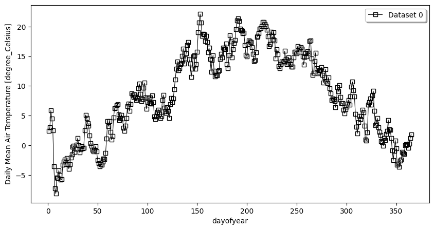
pyku.analyse.daily_mean(*dats, var=None, ax=None, **kwargs)[source]#

Daily mean

Parameters:

dats (xarray.Dataset) – The input dataset(s)
var (str) – The variable name.
**kwargs – Any argument that can be passed to matplotlib.pyplot.figure() or matplotlib.pyplot.axes(). In particular ylim=(0,15), size_inches=(20, 40)), or yscale='log' can be passed.

Example

In [1]: %%time
   ...: import pyku
   ...: ds = pyku.resources.get_test_data('hyras_tas').compute()
   ...: ds.ana.daily_mean(var='tas')
   ...: 
CPU times: user 2.15 s, sys: 422 ms, total: 2.57 s
Wall time: 2.07 s

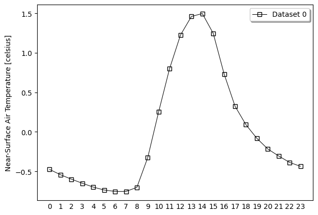
pyku.analyse.diurnal_cycle(*dats, var=None, ax=None, **kwargs)[source]#

Diurnal cycle

Parameters:

dats ([xarray.Dataset, List[xarray.Dataset]]) – The input dataset(s)
var (str) – The variable name.
**kwargs – Any argument that can be passed to matplotlib.pyplot.figure() or matplotlib.pyplot.axes(). In particular ylim=(0,15), size_inches=(20, 40)), or yscale='log' can be passed.

Example

In [1]: %%time
   ...: import pyku
   ...: ds = pyku.resources.get_test_data('hourly-tas').compute()
   ...: ds.ana.diurnal_cycle(var='tas')
   ...: 
CPU times: user 8.31 s, sys: 9.73 s, total: 18 s
Wall time: 16.5 s

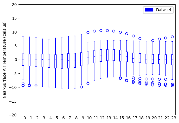
pyku.analyse.diurnal_cycle_variability(dat1, dat2=None, var=None, ax=None, **kwargs)[source]#

Diurnal cycle variability

Parameters:

dat1 (xarray.Dataset) – The first dataset.
dat2 (xarray.Dataset) – Optional. The second dataset.
var (str) – The variable name.
**kwargs – Any argument that can be passed to matplotlib.pyplot.figure() or func:matplotlib.pyplot.axes. In particular ylim=(0,15), size_inches=(20, 40)), or yscale='log' can be passed.

Example

In [1]: %%time
   ...: import pyku
   ...: ds = pyku.resources.get_test_data('hourly-tas')
   ...: ds.ana.diurnal_cycle_variability(var='tas', ylim=(-20, 20))
   ...: 
CPU times: user 5.79 s, sys: 1.64 s, total: 7.44 s
Wall time: 5.47 s

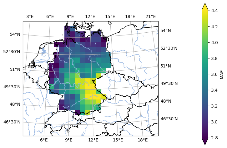
pyku.analyse.mae_map(*dats, ref=None, var=None, crs=None, **kwargs)[source]#

Map of the mean absolute error.

Parameters:

dats (xarray.Dataset) – The input dataset(s).
ref (xarray.Dataset) – The reference dataset.
var (str) – The variable name.
crs (cartopy.crs.CRS) – The coordinate reference system.
**kwargs – Any argument that can be passed to matplotlib.pyplot.pcolormesh(), matplotlib.pyplot.axes() matplotlib.pyplot.figure(), or cartopy.mpl.gridliner.gridlines(). For example, cmap, vmin, vmax, or size_inches can be passed.

Notes

If an argument is passed which is not recognized, no error message is thrown and the argument is ignored.

Example

In [1]: %%time
   ...: import pyku
   ...: 
   ...: # Open reference dataset and preprocess as needed
   ...: # -----------------------------------------------
   ...: 
   ...: ref = pyku.resources.get_test_data('hyras')\
   ...:       .pyku.to_cmor_units()\
   ...:       .pyku.set_time_labels_from_time_bounds(how='lower')\
   ...:       .pyku.project('HYR-LAEA-50')\
   ...:       .sel(time='1981')\
   ...:       .compute()
   ...: 
   ...: # Open model dataset and preprocess as needed
   ...: # -------------------------------------------
   ...: 
   ...: ds = pyku.resources.get_test_data('model_data')\
   ...:      .pyku.project('HYR-LAEA-50')\
   ...:      .pyku.set_time_labels_from_time_bounds(how='lower')\
   ...:      .sel(time='1981')\
   ...:      .compute()
   ...: 
   ...: # Calculate and plot
   ...: # ------------------
   ...: 
   ...: ds.ana.mae_map(ref=ref, var='tas', crs='HYR-LAEA-5')
   ...: 
CPU times: user 3.34 s, sys: 1.57 s, total: 4.91 s
Wall time: 7.33 s

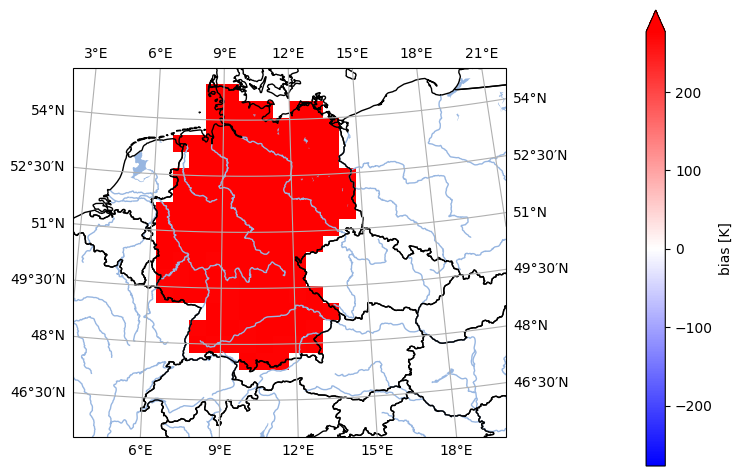
pyku.analyse.mean_bias_map(*dats, ref, var=None, crs=None, **kwargs)[source]#

Map of the mean bias

Parameters:

dats (xarray.Dataset, List[xarray.Dataset]) – The input model dataset(s)
ref (xarray.Dataset) – The Reference/Observation data
var (str) – The variable name
crs (cartopy.crs.CRS, pyresample.geometry.AreaDefinition, str) – Optional. The plot coordinate reference system.
**kwargs – Any argument that can be passed to matplotlib.pyplot.pcolormesh(), matplotlib.pyplot.axes() matplotlib.pyplot.figure(), or cartopy.mpl.gridliner.gridlines(). For example, cmap, vmin, vmax, or size_inches can be passed.

Notes

If an argument is passed which is not recognized, no error message is thrown and the argument is ignored.

Example

In [1]: %%time
   ...: import pyku
   ...: 
   ...: # Open reference dataset and preprocess as needed
   ...: # -----------------------------------------------
   ...: 
   ...: ref = pyku.resources.get_test_data('hyras')\
   ...:       .pyku.project('HYR-LAEA-50')\
   ...:       .sel(time='1981')\
   ...:       .compute()
   ...: 
   ...: # Open model dataset and preprocess as needed
   ...: # -------------------------------------------
   ...: 
   ...: ds = pyku.resources.get_test_data('model_data')\
   ...:      .pyku.project('HYR-LAEA-50')\
   ...:      .sel(time='1981')\
   ...:      .compute()
   ...: 
   ...: # Calculate and plot
   ...: # ------------------
   ...: 
   ...: ds.ana.mean_bias_map(dats=ds, ref=ref, var='tas', crs='HYR-LAEA-5')
   ...: 
CPU times: user 968 ms, sys: 293 ms, total: 1.26 s
Wall time: 930 ms

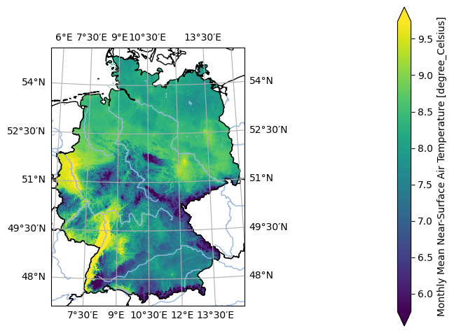
pyku.analyse.mean_map(*dats, var=None, crs=None, same_datetimes=True, **kwargs)[source]#

Map of the mean

Parameters:

dats (xarray.Dataset, List[xarray.Dataset]) – The input dataset(s)
var (str) – The variable name.
crs (cartopy.crs.CRS, pyresample.geometry.AreaDefinition, str) – (Optional) Coordinate reference system of the plot.
same_datetimes (bool) – (Optional) Defaults to True. Select common datetimes between datasets.
**kwargs – Any argument that can be passed to matplotlib.pyplot.pcolormesh(), matplotlib.pyplot.axes() matplotlib.pyplot.figure(), or cartopy.mpl.gridliner.gridlines(). For example, cmap, vmin, vmax, or size_inches can be passed.

Example

In [1]: %%time
   ...: import pyku
   ...: ds = (
   ...:     pyku.resources.get_test_data('hyras-tas-monthly')
   ...:     .compute()
   ...: )
   ...: ds.ana.mean_map(var='tas', crs='HYR-LAEA-5')
   ...: 
CPU times: user 653 ms, sys: 243 ms, total: 896 ms
Wall time: 744 ms

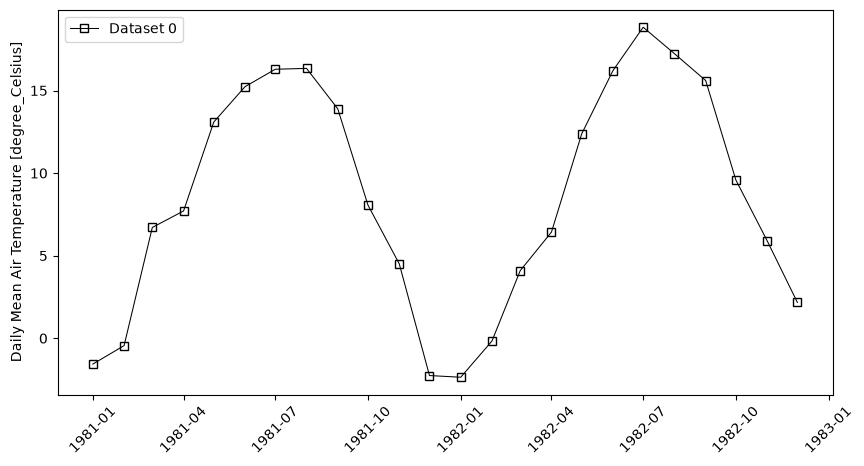
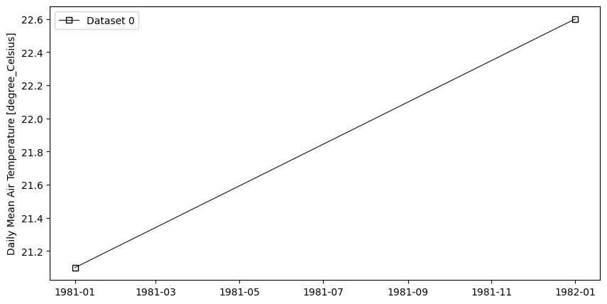
pyku.analyse.mean_vs_time(*dats, var=None, time_resolution='1YS', ax=None, **kwargs)[source]#

Mean vs time

Parameters:

*dats (xarray.Dataset, List[xarray.Dataset]) – The input dataset(s).
time_resolution (freqstr) – Time resolution (e.g. ‘1M’ or ‘6D’)
var (str) – The variable name.
ax (matplotlib.pyplot.axes) – Optional. Matplotlib pyplot axis.
**kwargs – Any argument that can be passed to matplotlib.pyplot.figure() or matplotlib.pyplot.axes(). In particular ylim=(0,15), size_inches=(20, 40)), or yscale='log' can be passed.

Example

In [1]: %%time
   ...: import pyku
   ...: ds = pyku.resources.get_test_data('hyras')
   ...: ds.ana.mean_vs_time(var='tas', time_resolution='1M')
   ...: 
CPU times: user 2.82 s, sys: 375 ms, total: 3.19 s
Wall time: 3.21 s

pyku.analyse.metadata(ds_mod, ds_obs)[source]#

Report on metadata

Parameters:

ds_mod (xarray.Dataset) – Model dataset.
ds_obs (xarray.Dataset) – Reference dataset.

Returns:

reStructuredText report

Return type:

str

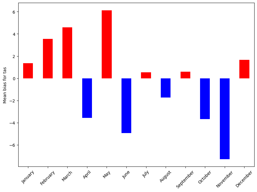
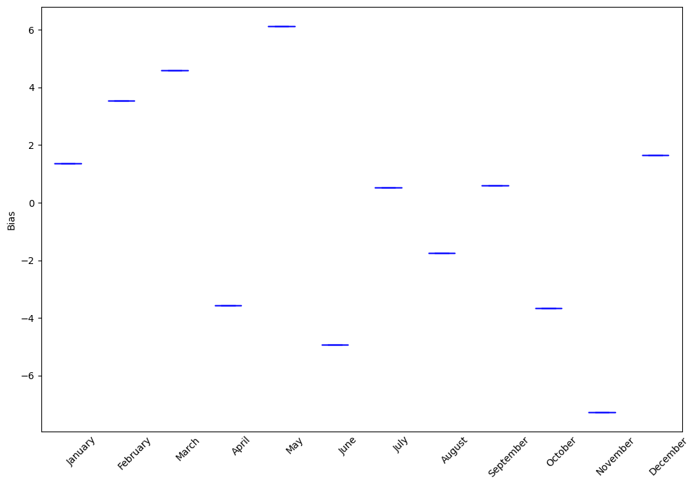
pyku.analyse.monthly_bias(dat_mod, dat_obs, var=None, ax=None, **kwargs)[source]#

Monthly bias

Parameters:

dat_mod (xarray.Dataset) – The input dataset.
dat_obs (xarray.Dataset) – The reference dataset.
var (str) – The variable name.
**kwargs – Any argument that can be passed to matplotlib.pyplot.figure() or matplotlib.pyplot.axes(). In particular ylim=(0,15), size_inches=(20, 40)), or yscale='log' can be passed.

Example

In [1]: import pyku
   ...: 
   ...: # Open reference data and preprocess as needed
   ...: # --------------------------------------------
   ...: 
   ...: ref = pyku.resources.get_test_data('hyras')\
   ...:      .pyku.to_cmor_units()\
   ...:      .pyku.set_time_labels_from_time_bounds(how='lower')\
   ...:      .pyku.project('HYR-LAEA-50')\
   ...:      .sel(time='1981')\
   ...:      .compute()
   ...: 
   ...: # Open model data and preprocess as needed
   ...: # ----------------------------------------
   ...: 
   ...: ds = pyku.resources.get_test_data('model_data')\
   ...:      .pyku.project('HYR-LAEA-50')\
   ...:      .pyku.set_time_labels_from_time_bounds(how='lower')\
   ...:      .sel(time='1981')\
   ...:      .compute()
   ...: 
   ...: # Calculate and plot
   ...: # ------------------
   ...: 
   ...: ds.ana.monthly_bias(ref, var='tas')
   ...: 

pyku.analyse.monthly_bias_var(ds_mod, ds_obs, var, **kwargs)[source]#

Monthly bias variation

Parameters:

ds_mod (xarray.Dataset) – The input dataset.
ds_obs (xarray.Dataset) – The reference dataset.
var (str) – The variable name.
crs (cartopy.crs.CRS, pyresample.geometry.AreaDefinition) – (Optional) Coordinate reference system of the plot.
**kwargs – Any argument that can be passed to matplotlib.pyplot.figure() or matplotlib.pyplot.axes(). In particular ylim=(0,15), size_inches=(20, 40)), or yscale='log' can be passed.

Example

In [1]: %%time
   ...: import pyku
   ...: 
   ...: # Open, reproject
   ...: # ---------------
   ...: 
   ...: ref = pyku.resources.get_test_data('hyras')\
   ...:      .pyku.set_time_labels_from_time_bounds(how='lower')\
   ...:      .pyku.to_cmor_units()\
   ...:      .pyku.project('HYR-LAEA-50')\
   ...:      .sel(time='1981')
   ...: 
   ...: # Open model, reproject, reset time labels, select the year
   ...: # ---------------------------------------------------------
   ...: 
   ...: ds = pyku.resources.get_test_data('model_data')\
   ...:      .pyku.project('HYR-LAEA-50')\
   ...:      .pyku.set_time_labels_from_time_bounds(how='lower')\
   ...:      .sel(time='1981')
   ...: 
   ...: # Calculate and plot
   ...: # ------------------
   ...: 
   ...: ds.ana.monthly_bias_var(ref, var='tas')
   ...: 
CPU times: user 1.55 s, sys: 333 ms, total: 1.88 s
Wall time: 1.21 s

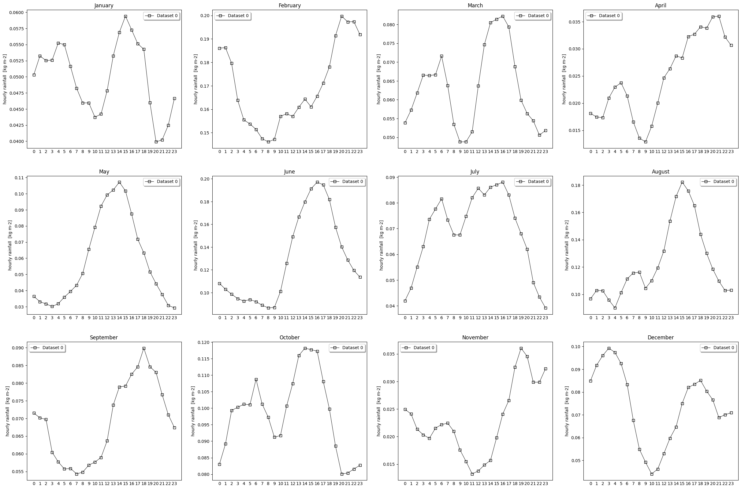
pyku.analyse.monthly_diurnal_cycle(dat1, dat2=None, var=None, ax=None, **kwargs)[source]#

Diurnal cycle mean for each month

Parameters:

ds_mod (xarray.Dataset) – The input dataset.
ds_obs (xarray.Dataset) – Optional. The second dataset.
var (str) – variable name
**kwargs – Any argument that can be passed to matplotlib.pyplot.figure() or matplotlib.pyplot.axes(). In particular ylim=(0,15), size_inches=(20, 40)), or yscale='log' can be passed.

Example

In [1]: %%time
   ...: import pyku
   ...: ds = pyku.resources.get_test_data('low-res-hourly-tas-data')
   ...: ds = ds.compute()
   ...: ds.ana.monthly_diurnal_cycle(var='RR')
   ...: 
CPU times: user 8.63 s, sys: 6.2 s, total: 14.8 s
Wall time: 13 s

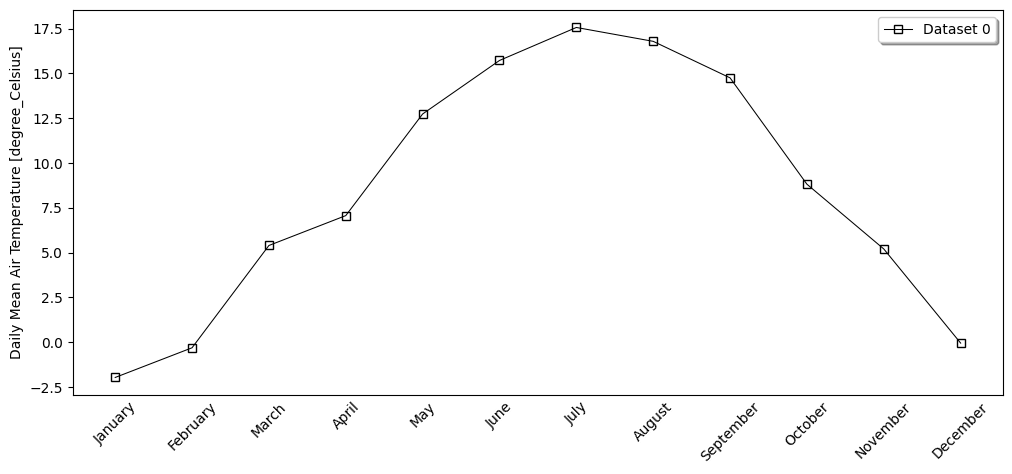
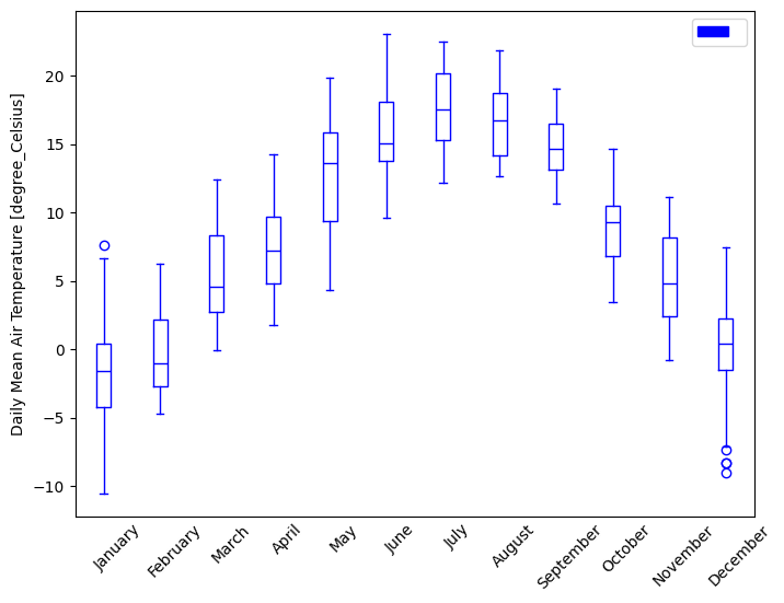
pyku.analyse.monthly_mean(*dats, var=None, **kwargs)[source]#

Monthly mean

Parameters:

dats (Union[xarray.Dataset, List[xarray.Dataset]]) – The input dataset(s)
var (str) – The variable name.
**kwargs – Any argument that can be passed to matplotlib.pyplot.figure() or matplotlib.pyplot.axes(). In particular ylim=(0,15), size_inches=(20, 40)), or yscale='log' can be passed.

Example

In [1]: %%time
   ...: import pyku
   ...: ds = pyku.resources.get_test_data('hyras_tas')
   ...: ds.ana.monthly_mean(var='tas')
   ...: 
CPU times: user 680 ms, sys: 194 ms, total: 874 ms
Wall time: 877 ms

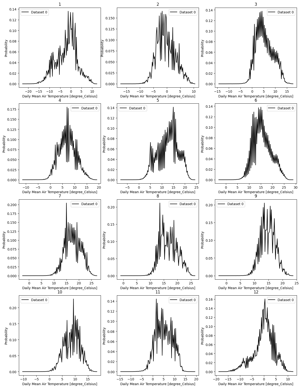
pyku.analyse.monthly_pdf(*dats, var=None, **kwargs)[source]#

Probability distribution function for each season

Parameters:

*dats (xarray.Dataset, List[xarray.Dataset]) – The input dataset(s)
var (str) – The variable name.
crs (cartopy.crs.CRS, pyresample.geometry.AreaDefinition, str) – (Optional). The coordinate reference system of the plot.
**kwargs – Any argument that can be passed to matplotlib.pyplot.figure() or matplotlib.pyplot.axes(). In particular ylim=(0,15), size_inches=(20, 40)), or yscale='log' can be passed.

Example

In [1]: %%time
   ...: import pyku
   ...: ds = pyku.resources.get_test_data('hyras_tas').compute()
   ...: ds.ana.monthly_pdf(var='tas')
   ...: 
CPU times: user 2.84 s, sys: 2.54 s, total: 5.38 s
Wall time: 5.21 s

pyku.analyse.monthly_variability(dat1, dat2=None, var=None, ax=None, **kwargs)[source]#

Monthly variability

Parameters:

dat1 (xarray.Dataset) – The first dataset.
dat2 (xarray.Dataset) – Optional. The second dataset.
var (str) – The variable name.
**kwargs – Any argument that can be passed to matplotlib.pyplot.figure() or matplotlib.pyplot.axes(). In particular ylim=(0,15), size_inches=(20, 40)), or yscale='log' can be passed.

Example

In [1]: import pyku
   ...: ds = pyku.resources.get_test_data('hyras_tas').compute()
   ...: ds.ana.monthly_variability(var='tas', size_inches=(8, 6))
   ...: 

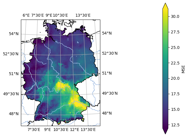
pyku.analyse.mse_map(*dats, ref, var=None, ds_ref=None, crs=None, **kwargs)[source]#

Map of the Mean Squared Error (MSE)

Parameters:

dats ([xarray.Dataset, List[xarray.Dataset]) – The input dataset(s).
ref (xarray.Dataset) – The reference dataset.
var (str) – The variable name.
crs (cartopy.crs.CRS, pyresample.geometry.AreaDefinition, str) – Optional. The coordinate reference system of the plot.
**kwargs – Any argument that can be passed to matplotlib.pyplot.pcolormesh(), matplotlib.pyplot.axes() matplotlib.pyplot.figure(), or cartopy.mpl.gridliner.gridlines(). For example, cmap, vmin, vmax, or size_inches can be passed.

Example

In [1]: %%time
   ...: import pyku
   ...: 
   ...: # Open reference dataset and preprocess as needed
   ...: # -----------------------------------------------
   ...: 
   ...: ref = (
   ...:     pyku.resources.get_test_data('hyras')
   ...:     .pyku.to_cmor_units()
   ...:     .pyku.set_time_labels_from_time_bounds(how='lower')
   ...:     .pyku.project('HYR-GER-LAEA-5')
   ...:     .sel(time='1981')
   ...:     .compute()
   ...: )
   ...: 
   ...: # Open model dataset and preprocess as needed
   ...: # -------------------------------------------
   ...: 
   ...: ds = (
   ...:     pyku.resources.get_test_data('model_data')
   ...:     .pyku.project('HYR-GER-LAEA-5')
   ...:     .pyku.set_time_labels_from_time_bounds(how='lower')
   ...:     .sel(time='1981')
   ...:     .compute()
   ...: )
   ...: 
   ...: # Calculate and plot
   ...: # ------------------
   ...: 
   ...: ds.ana.mse_map(ref=ref, var='tas', crs='HYR-GER-LAEA-5')
   ...: 
CPU times: user 1.16 s, sys: 354 ms, total: 1.51 s
Wall time: 1.11 s

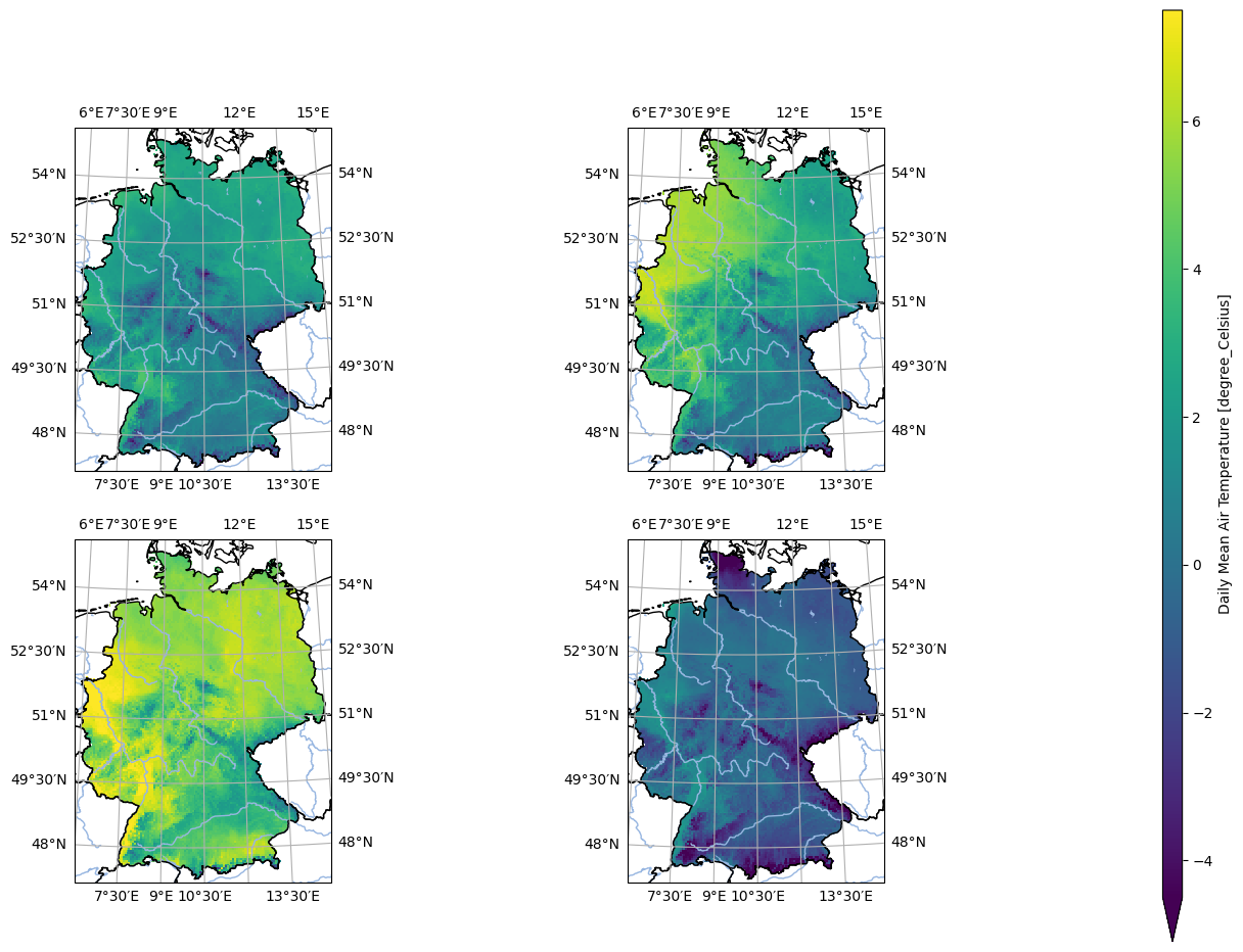
pyku.analyse.n_maps(*dats, var=None, crs=None, colorbar=True, **kwargs)[source]#

Plot n maps side by side

Parameters:

dats (xarray.Dataset, or List[xarray.Dataset]) – The input dataset.
var (str) – The variable name
crs (cartopy.crs.CRS, pyresample.geometry.AreaDefinition, str) – (Optional) Coordinate reference system of the plot. If a string is passed, a pre-configured projection definition is taken from the configuration files (e.g. ‘EUR-44’, ‘HYR-LAEA-5’).
colorbar (bool) – Optional. Defaults to True. If set to False, the colorbar is not shown and the colormap of all plots is set independently.
**kwargs – Any argument that can be passed to matplotlib.pyplot.pcolormesh(), matplotlib.pyplot.axes() matplotlib.pyplot.figure(), or cartopy.mpl.gridliner.gridlines(). For example, cmap, vmin, vmax, or size_inches can be passed. Further options to control the layout: wspace (value for plt.subplots_adjust),

Example

In [1]: %%time
   ...: import pyku
   ...: 
   ...: ds = (
   ...:     pyku.resources.get_test_data('small_tas_dataset')
   ...:     .compute()
   ...: )
   ...: 
   ...: pyku.analyse.n_maps(
   ...:     ds.isel(time=0),
   ...:     ds.isel(time=1),
   ...:     ds.isel(time=2),
   ...:     ds.isel(time=3),
   ...:     nrows=2,
   ...:     ncols=2,
   ...:     var='tas',
   ...:     crs='HYR-GER-LAEA-5'
   ...: )
   ...: 
CPU times: user 328 ms, sys: 257 ms, total: 585 ms
Wall time: 380 ms

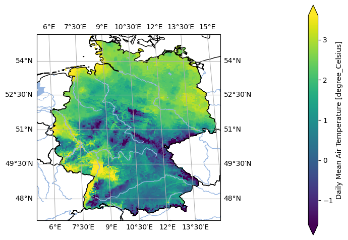
pyku.analyse.one_map(dat, var=None, crs=None, **kwargs)[source]#

Plot one map

Parameters:

dat (xarray.Dataset) – The input dataset.
var (str) – The name of the variable.
crs (Union[cartopy.crs.CRS, pyresample.geometry.AreaDefinition, str]) – Coordinate reference system. A pyku pre-defined projection identifier can be passed with a string.
**kwargs – Any argument that can be passed to matplotlib.pyplot.pcolormesh(), matplotlib.pyplot.axes(), matplotlib.pyplot.figure(), or cartopy.mpl.geoaxes.GeoAxes.gridlines(). For example, cmap, vmin, vmax, or size_inches can be passed.

Example

In [1]: %%time
   ...: import pyku
   ...: ds = (
   ...:    pyku.resources.get_test_data('small_tas_dataset')
   ...:    .isel(time=0).compute()
   ...: )
   ...: ds.ana.one_map(var='tas', crs='seamless_world')
   ...: 
CPU times: user 219 ms, sys: 199 ms, total: 419 ms
Wall time: 271 ms

pyku.analyse.p98_map(*dats, var, crs=None, **kwargs)[source]#

Map of the 98th percentile

Parameters:

*dats ([xarray.Dataset, List[:class:`xarray.Dataset]]) – The input dataset(s)
var (str) – The variable name.
crs (cartopy.crs.CRS, pyresample.geometry.AreaDefinition, str) – Optional. The coordinate reference system of the plot.
**kwargs – Any argument that can be passed to matplotlib.pyplot.pcolormesh(), matplotlib.pyplot.axes() matplotlib.pyplot.figure(), or cartopy.mpl.gridliner.gridlines(). For example, cmap, vmin, vmax, or size_inches can be passed.

pyku.analyse.p98_vs_time(*dats, var=None, time_resolution='1YS', ax=None, **kwargs)[source]#

98th percentile vs time

Parameters:

*dats ([xarray.Dataset, List[xarray.Dataset]]) – The input dataset(s).
time_resolution (str) – The time resolution, e.g. ‘1MS’ or ‘6D’.
var (str) – The variable name.
( (ax) – class:matplotlib.pyplot.axes): Optional. Matplotlib pyplot axis.
**kwargs – Any argument that can be passed to matplotlib.pyplot.figure() or matplotlib.pyplot.axes(). In particular ylim=(0,15), size_inches=(20, 40)), or yscale='log' can be passed.

Example

In [1]: %%time
   ...: import pyku
   ...: ds = pyku.resources.get_test_data('hyras_tas')
   ...: ds.ana.p98_vs_time(var='tas')
   ...: 
CPU times: user 485 ms, sys: 157 ms, total: 642 ms
Wall time: 642 ms

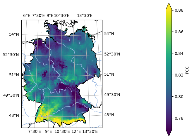
pyku.analyse.pcc_map(*dats, ref, var=None, crs=None, **kwargs)[source]#

Map of the Pearson Correlation Coefficient (PCC)

Parameters:

dats ([xarray.Dataset, List[xarray.Datasets]]) – The input dataset(s)
ref (xarray.Dataset) – The reference dataset.
var (str) – Variable name
crs (cartopy.crs.CRS, pyresample.geometry.AreaDefinition, str) – Optional. The coordinate reference system of the plot.
**kwargs – Any argument that can be passed to matplotlib.pyplot.pcolormesh(), matplotlib.pyplot.axes() matplotlib.pyplot.figure(), or cartopy.mpl.gridliner.gridlines(). For example, cmap, vmin, vmax, or size_inches can be passed.

Example

In [1]: %%time
   ...: import pyku
   ...: 
   ...: # Open reference dataset and preprocess as needed
   ...: # -----------------------------------------------
   ...: 
   ...: ref = (
   ...:     pyku.resources.get_test_data('hyras')
   ...:     .pyku.to_cmor_units()
   ...:     .pyku.set_time_labels_from_time_bounds(how='lower')
   ...:     .pyku.project('HYR-GER-LAEA-5')
   ...:     .sel(time='1981')
   ...:     .compute()
   ...: )
   ...: 
   ...: # Open model dataset and preprocess as needed
   ...: # -------------------------------------------
   ...: 
   ...: ds = (
   ...:     pyku.resources.get_test_data('model_data')
   ...:     .pyku.project('HYR-GER-LAEA-5')
   ...:     .pyku.set_time_labels_from_time_bounds(how='lower')
   ...:     .sel(time='1981')
   ...:     .compute()
   ...: )
   ...: 
   ...: # Calculate and plot
   ...: # ------------------
   ...: 
   ...: ds.ana.pcc_map(ref=ref, var='tas', crs='HYR-GER-LAEA-5')
   ...: 
CPU times: user 1.15 s, sys: 380 ms, total: 1.53 s
Wall time: 1.13 s

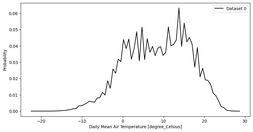
pyku.analyse.pdf(*dats, var=None, ax=None, **kwargs)[source]#

Probability distribution function

Parameters:

dats ([xarray.Dataset, List[xarray.DataArray]]) – The input dataset(s)
var (str) – The variable names.
**kwargs – Any argument that can be passed to matplotlib.pyplot.figure or matplotlib.pyplot.axes(). In particular ylim=(0,15), size_inches=(20, 40)), or yscale='log' can be passed.
range (tuple) – data Range, e.g. range=(0, 10).
nbins (int) – Number of bins.
nsamples (int) – Number of points sampled from the data..

Example

In [1]: %%time
   ...: import pyku
   ...: ds = pyku.resources.get_test_data('hyras_tas').compute()
   ...: ds.ana.pdf(var='tas', nbins=80)
   ...: 
CPU times: user 338 ms, sys: 111 ms, total: 449 ms
Wall time: 445 ms

pyku.analyse.pdf2D(ds, var=None, varx=None, vary=None, sample_size=100, ax=None, **kwargs)[source]#

2D distribution

Parameters:

ds (xarray.Dataset) – The input dataset.
varx (str) – The variable on the x axis.
vary (str) – The variable on the y axis.
sample_size (int) – The sample size.
**kwargs – Any argument that can be passed to matplotlib.pyplot.figure() or matplotlib.pyplot.axes(). In particular ylim=(0,15), size_inches=(20, 40)), or yscale='log' can be passed.

pyku.analyse.percentile_map(ds_mod, ds_obs, var=None, percentile=0.5, crs=None, **kwargs)[source]#

Map of the nth percentile

Todo

Check if function is actually working
Create a documentation
I think the CRS should also work with pyresample.geometry.AreaDefinition.

Parameters:

ds_mod (xarray.Dataset) – The first dataset.
ds_obs (xarray.Dataset) – The second dataset.
var (str) – Variable name
percentile (float) – Percentile between 0 and 1
crs (cartopy.crs.CRS) – Coordinate reference system

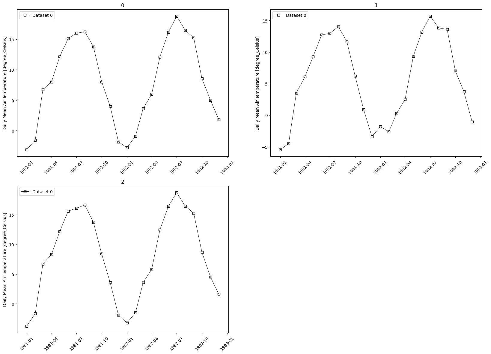
pyku.analyse.regional_mean_vs_time(ds_mod, ds_obs=None, gdf=None, time_resolution='1MS', var=None, **kwargs)[source]#

Time series per region

Parameters:

ds_mod (xarray.Dataset) – The first input dataset.
ds_obs (xarray.Dataset) – The second input dataset.
gdf (geopandas.GeoDataFrame) – The polygon data.
var (str) – variable name
**kwargs – Any argument that can be passed to matplotlib.pyplot.figure() or matplotlib.pyplot.axes(). In particular ylim=(0,15), size_inches=(20, 40)), or yscale='log' can be passed.

Examples

In [1]: %%time
   ...: import xarray as xr
   ...: import pyku
   ...: import pyku.analyse as analyse
   ...: 
   ...: # Open and preprocess test data as needed
   ...: # ---------------------------------------
   ...: 
   ...: ds = pyku.resources.get_test_data('hyras')
   ...: 
   ...: # Get a subset ot the natrual areas or germany
   ...: # --------------------------------------------
   ...: 
   ...: regions = (
   ...:     pyku.resources
   ...:     .get_geodataframe('natural_areas_of_germany')
   ...:     .head(3)
   ...: )
   ...: 
   ...: ds.ana.regional_mean_vs_time(
   ...:     gdf=regions,
   ...:     time_resolution='1MS',
   ...:     var='tas'
   ...: )
   ...: 
CPU times: user 11.6 s, sys: 2.1 s, total: 13.7 s
Wall time: 13.6 s

pyku.analyse.regional_monthly_bias(ds_mod, ds_obs, gdf, area_def, var=None, **kwargs)[source]#

Monthly variability

Todo

Check if this function is working
Get the ipython code right
Check documentation is right. I think area_def can be passed as cartopy crs?

Parameters:

ds_mod (xarray.Dataset) – The first input dataset.
ds_obs (xarray.Dataset) – The second input dataset.
gdf (geopandas.GeoDataFrame) – The polygon data.
var (str) – variable name
area_def (pyresample.geometry.AreaDefinition) – Optional. The plot coordinate reference system.
**kwargs – Any argument that can be passed to matplotlib.pyplot.figure() or matplotlib.pyplot.axes(). In particular ylim=(0,15), size_inches=(20, 40)), or yscale='log' can be passed.

Examples

In [1]: %%time
   ...: import pyku
   ...: 
   ...: # Open reference data and preprocess as needed
   ...: # --------------------------------------------
   ...: 
   ...: ref = (
   ...:     pyku.resources.get_test_data('hyras')
   ...:     .pyku.to_cmor_units()
   ...:     .pyku.set_time_labels_from_time_bounds(how='lower')
   ...:     .pyku.project('HYR-LAEA-50')
   ...:     .sel(time='1981')
   ...:     .compute()
   ...: )
   ...: 
   ...: # Open model data and preprocess as needed
   ...: # ----------------------------------------
   ...: 
   ...: ds = (
   ...:     pyku.resources.get_test_data('model_data')
   ...:     .pyku.project('HYR-LAEA-50')
   ...:     .pyku.set_time_labels_from_time_bounds(how='lower')
   ...:     .sel(time='1981')
   ...:     .compute()
   ...: )
   ...: 
   ...: gdf = (
   ...:     pyku.resources
   ...:     .get_geodataframe('natural_areas_of_germany')
   ...:     .loc[0:4]
   ...: )
   ...: 
   ...: print('Polygons: ', gdf)
   ...: 
   ...: # Calculate and plot
   ...: # ------------------
   ...: 
   ...: # pyku.analyse.regional_monthly_bias(
   ...: #     ds, ref, gdf, area_def='HYR-LAEA-50', var='tas'
   ...: # )
   ...: 
Polygons:       Shape_Leng  ...                                           geometry
0  1.676004e+06  ...  POLYGON ((3613725.5 5598209, 3613437 5597195, ...
1  8.566480e+05  ...  MULTIPOLYGON (((3614073 5273052, 3614476 52725...
2  1.096050e+06  ...  POLYGON ((3734247 5437391, 3734470 5437339, 37...
3  9.577557e+05  ...  POLYGON ((3288568.5 5633985.5, 3288857.25 5633...
4  1.457899e+06  ...  MULTIPOLYGON (((3794440.445 6030118.175, 37943...

[5 rows x 12 columns]
CPU times: user 870 ms, sys: 183 ms, total: 1.05 s
Wall time: 819 ms

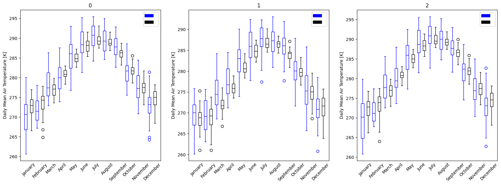
pyku.analyse.regional_monthly_variability(ds1, ds2, gdf=None, var=None, **kwargs)[source]#

Monthly variability

Parameters:

ds1 (xarray.Dataset) – The first dataset.
ds2 (xarray.Dataset) – The second dataset.
gdf (geopandas.GeoDataFrame) – The polygon data.
var (str) – The variable name.
**kwargs – Any argument that can be passed to matplotlib.pyplot.figure() or matplotlib.pyplot.axes(). In particular ylim=(0,15), size_inches=(20, 40)), or yscale='log' can be passed.

Examples

In [1]: import xarray as xr
   ...: import pyku
   ...: import pyku.analyse as analyse
   ...: 
   ...: # Open and preprocess test data as needed
   ...: # ---------------------------------------
   ...: 
   ...: ds1 = (
   ...:     pyku.resources.get_test_data('hyras')
   ...:     .pyku.to_cmor_varnames()
   ...:     .pyku.to_cmor_units()
   ...: )
   ...: 
   ...: ds2 = pyku.resources.get_test_data('cordex_data')
   ...: 
   ...: # Get a subset ot the natrual areas or germany
   ...: # --------------------------------------------
   ...: 
   ...: regions = (
   ...:     pyku.resources
   ...:     .get_geodataframe('natural_areas_of_germany')
   ...:    .head(3)
   ...:  )
   ...: 
   ...: # Calculate and plot
   ...: # ------------------
   ...: 
   ...: analyse.regional_monthly_variability(
   ...:     ds1,
   ...:     ds2,
   ...:     gdf=regions,
   ...:     var='tas'
   ...: )
   ...: 

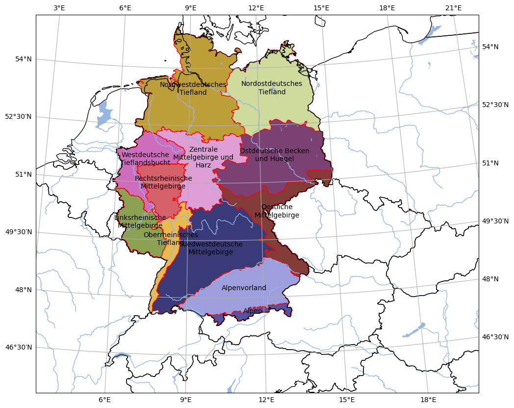
_images/regional_monthly_variability.png

pyku.analyse.regions(gdf, area_def, **kwargs)[source]#

Plot regions

Parameters:

gdf (geopandas.GeoDataFrame) – Polygon data
area_def ([pyresample.AreaDefinition, string]) – Area definition
**kwargs – Any argument that can be passed to matplotlib.Artist In particular size_inches can be passed.

Example

In [1]: import pyku
   ...: gdf = pyku.resources.get_geodataframe(
   ...:     'natural_areas_of_germany'
   ...: )
   ...: pyku.analyse.regions(gdf, area_def='HYR-LAEA-5')
   ...: 

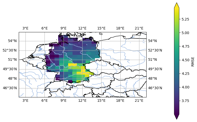
pyku.analyse.rmse_map(*dats, ref, var=None, crs=None, ds_ref=None, **kwargs)[source]#

Map of the Root Mean Squared Error (RMSE)

Parameters:

dats ([xarray.Dataset, List[xarray.Dataset]]) – The input dataset(s).
ref (xarray.Dataset) – The reference dataset.
var (str) – The variable name.
crs (cartopy.crs.CRS, pyresample.geometry.AreaDefinition, str) – Optional. The coordinate reference system of the plot.
**kwargs – Any argument that can be passed to matplotlib.pyplot.pcolormesh(), matplotlib.pyplot.axes() matplotlib.pyplot.figure(), or cartopy.mpl.gridliner.gridlines(). For example, cmap, vmin, vmax, or size_inches can be passed.

Example

In [1]: %%time
   ...: import pyku
   ...: 
   ...: # Open reference dataset and preprocess as needed
   ...: # -----------------------------------------------
   ...: 
   ...: ref = pyku.resources.get_test_data('hyras')\
   ...:       .pyku.to_cmor_units()\
   ...:       .pyku.set_time_labels_from_time_bounds(how='lower')\
   ...:       .pyku.project('HYR-LAEA-50')\
   ...:       .sel(time='1981')\
   ...:       .load()
   ...: 
   ...: # Open model dataset and preprocess as needed
   ...: # -------------------------------------------
   ...: 
   ...: ds = pyku.resources.get_test_data('model_data')\
   ...:      .pyku.project('HYR-LAEA-50')\
   ...:      .pyku.set_time_labels_from_time_bounds(how='lower')\
   ...:      .sel(time='1981')\
   ...:      .load()
   ...: 
   ...: # Calculate and plot
   ...: # ------------------
   ...: 
   ...: ds.ana.rmse_map(ref=ref, var='tas')
   ...: 
CPU times: user 1.02 s, sys: 377 ms, total: 1.39 s
Wall time: 941 ms

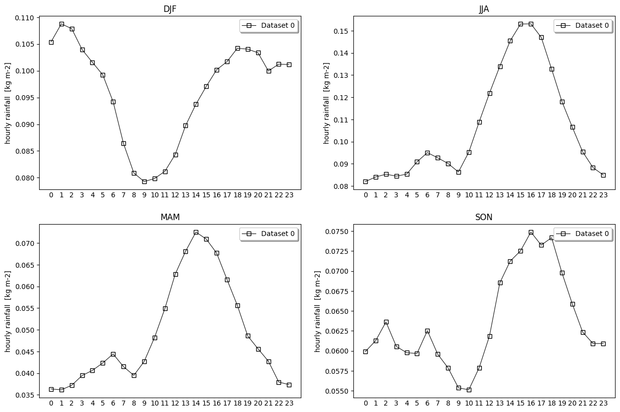
pyku.analyse.seasonal_diurnal_cycle(dat1, dat2=None, var=None, ax=None, **kwargs)[source]#

Diurnal cycle for each seasons

Parameters:

ds_mod (xarray.Dataset) – Model data
ds_obs (xarray.Dataset) – Reference data
var (str) – The variable name.
**kwargs – Any argument that can be passed to matplotlib.pyplot.figure() or matplotlib.pyplot.axes(). In particular ylim=(0,15), size_inches=(20, 40)), or yscale='log' can be passed.

Examples

In [1]: %%time
   ...: import pyku
   ...: ds = pyku.resources.get_test_data('low-res-hourly-tas-data')
   ...: ds.ana.seasonal_diurnal_cycle(var='RR')
   ...: 
CPU times: user 7.78 s, sys: 2.92 s, total: 10.7 s
Wall time: 8.76 s

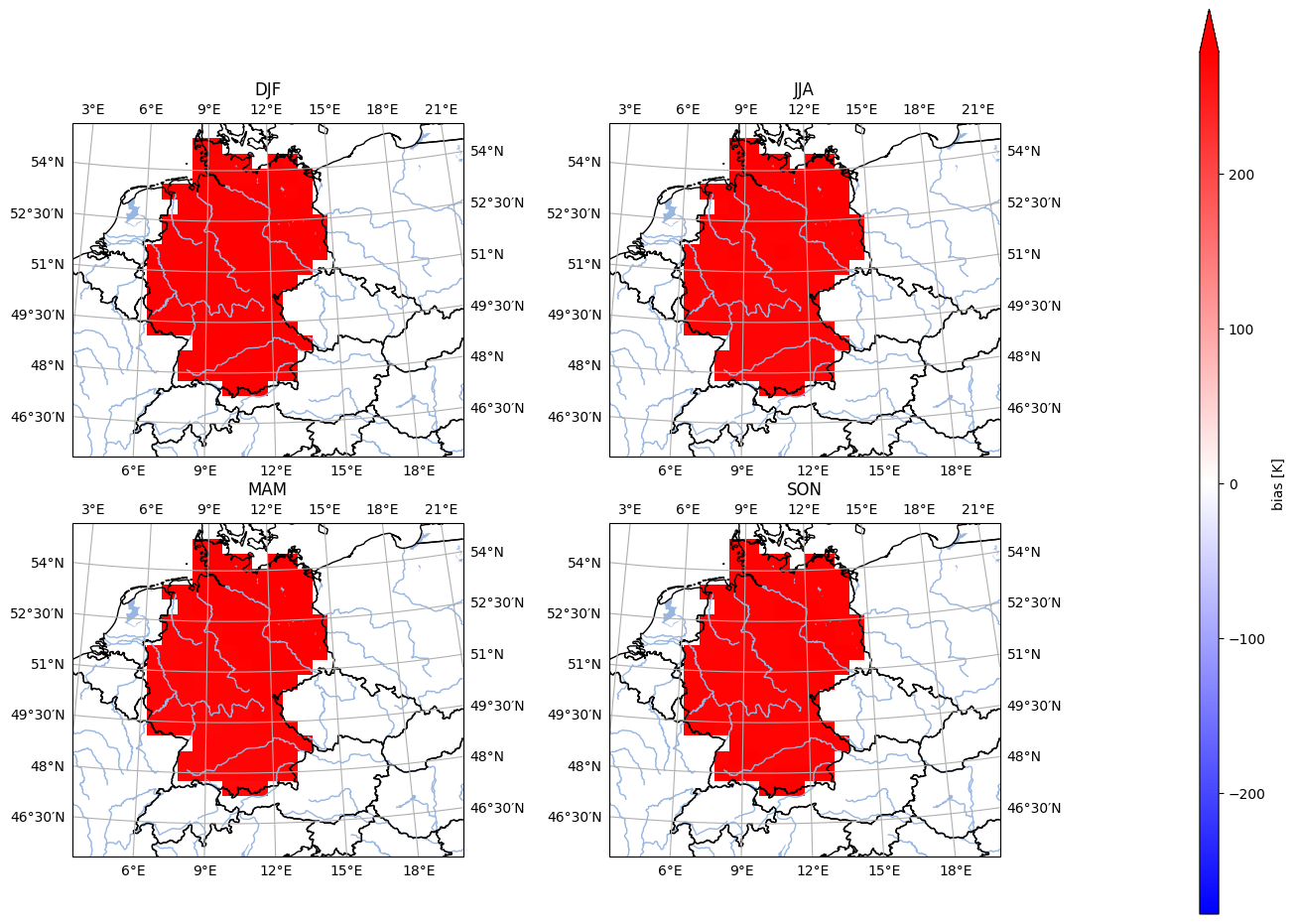
pyku.analyse.seasonal_mean_bias_map(dats, ref, var=None, crs=None, **kwargs)[source]#

Map of the mean bias

Parameters:

dats (xarray.Dataset) – The input model dataset
ref (xarray.Dataset) – The Reference/Observation data
var (str) – The variable name
crs (cartopy.crs.CRS, pyresample.geometry.AreaDefinition, str) – Optional. The plot coordinate reference system.
**kwargs – Any argument that can be passed to matplotlib.pyplot.pcolormesh(), matplotlib.pyplot.axes() matplotlib.pyplot.figure(), or cartopy.mpl.gridliner.gridlines(). For example, cmap, vmin, vmax, or size_inches can be passed.

Notes

If an argument is passed which is not recognized, no error message is thrown and the argument is ignored.

Example

In [1]: import pyku
   ...: 
   ...: # Open reference dataset and preprocess as needed
   ...: # -----------------------------------------------
   ...: 
   ...: ref = (
   ...:     pyku.resources.get_test_data('hyras')
   ...:     .pyku.project('HYR-LAEA-50')
   ...:     .sel(time='1981')
   ...:     .compute()
   ...: )
   ...: 
   ...: # Open model dataset and preprocess as needed
   ...: # -------------------------------------------
   ...: 
   ...: ds = (
   ...:     pyku.resources.get_test_data('model_data')
   ...:     .pyku.project('HYR-LAEA-50')
   ...:     .sel(time='1981')
   ...:     .compute()
   ...: )
   ...: 
   ...: # Calculate and plot
   ...: # ------------------
   ...: 
   ...: ds.ana.seasonal_mean_bias_map(
   ...:     ref=ref,
   ...:     var='tas',
   ...:     crs='HYR-LAEA-50'
   ...: )
   ...: 

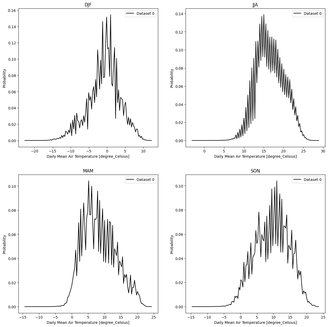
pyku.analyse.seasonal_pdf(*dats, var=None, **kwargs)[source]#

Probability distribution function for each season

Parameters:

dats (xarray.Dataset, List[xarray.Dataset]]) – The input dataset(s).
var (str) – The variable name.
**kwargs – Any argument that can be passed to matplotlib.pyplot.figure() or matplotlib.pyplot.axes(). In particular ylim=(0,15), size_inches=(20, 40)), or yscale='log' can be passed.

Example

In [1]: import pyku
   ...: ds = pyku.resources.get_test_data('hyras_tas')
   ...: ds.ana.seasonal_pdf(var='tas')
   ...: 

pyku.analyse.summary_table(ds_mod, ds_obs, **kwargs)[source]#

Summary in table form

Parameters:

ds_mod (xarray.Dataset) – Model dataset.
ds_obs (xarray.Dataset) – Reference dataset.

Returns:

reStructuredText table

Return type:

str

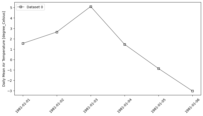
pyku.analyse.time_serie(*dats, var=None, ax=None, **kwargs)[source]#

Time serie. The data are averaged over y/x and plotting against time

Parameters:

*dats (xarray.Dataset, List[xarray.Dataset]) – The input dataset(s).
var (str) – The variable name.
ax (matplotlib.pyplot.axes) – Optional. Matplotlib pyplot axis.
**kwargs – Any argument that can be passed to matplotlib.pyplot.figure() or matplotlib.pyplot.axes(). In particular ylim=(0,15), size_inches=(20, 40)), or yscale='log' can be passed.

Example

In [1]: pyku
   ...: ds = pyku.resources.get_test_data('hyras_tas')\
   ...: .isel(time=[0,1,2,3,4,5])
   ...: ds.ana.time_serie(var='tas')
   ...: 

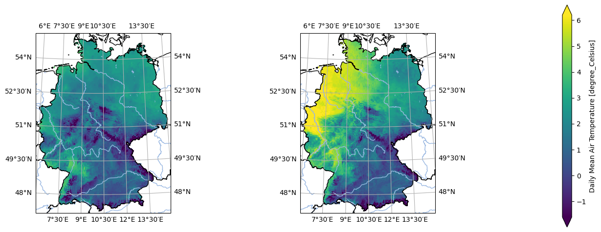
pyku.analyse.two_maps(dat1, dat2, var=None, crs=None, **kwargs)[source]#

Plot two maps side by side

Parameters:

dat1 (xarray.Dataset) – The first dataset.
dat2 (xarray.Dataset) – The second dataset.
var (str) – The name of the variable.
crs (Union[cartopy.crs.CRS, pyresample.geometry.AreaDefinition, str]) – Coordonate reference system. A pyku pre-defined projection identifier can be passed with a string.
**kwargs – Any argument that can be passed to matplotlib.pyplot.pcolormesh(), matplotlib.pyplot.axes() matplotlib.pyplot.figure(), or cartopy.mpl.geoaxes.GeoAxes.gridlines(). For example, cmap, vmin, vmax, or size_inches can be passed.

Notes

If an argument is passed which is not recognized, no error message is thrown and the argument is ignored.

Example

In [1]: %%time
   ...: import pyku
   ...: 
   ...: ds = pyku.resources.get_test_data('small_tas_dataset')
   ...: 
   ...: pyku.analyse.two_maps(
   ...:     ds.isel(time=0),
   ...:     ds.isel(time=1),
   ...:     rows=1,
   ...:     cols=2,
   ...:     var='tas',
   ...:     crs='HYR-GER-LAEA-5',
   ...: )
   ...: 
CPU times: user 253 ms, sys: 203 ms, total: 457 ms
Wall time: 284 ms

pyku.analyse.var_vs_year(dat_mod, dat_obs, var=None, **kwargs)[source]#

Variability vs year

Todo

Function looks very outdated and needs to be reworked

Parameters:

ds_mod (xarray.Dataset) – The first dataset.
ds_obs (xarray.Dataset) – The second dataset.
var (str) – Variable name
**kwargs – Any argument that can be passed to matplotlib.pyplot.figure() or matplotlib.pyplot.axes(). In particular ylim=(0,15), size_inches=(20, 40)), or yscale='log' can be passed.

pyku.analyse.wasserstein_distance(ds_mod, ds_obs, nsamples=10000, numItermax=500000)[source]#: Warning

This function is under construction

Wasserstein distance

pyku.analyse

Contents

pyku.analyse#