Geographic projections#
pyku provides standardized geographic projections, each identified by a unique string. These projections are named for easy reference. For instance, to view the new HYRAS LAEA grid at a 5 km resolution, you can use the following command:
[1]:
import pyku.geo as geo

area_def = geo.load_area_def('HYR-LAEA-5')
print(area_def)
Area ID: HYR-LAEA-5
Description: HYR-LAEA-5
Projection: {'ellps': 'GRS80', 'lat_0': '52', 'lon_0': '10', 'no_defs': 'None', 'proj': 'laea', 'towgs84': '[0.0, 0.0, 0.0, 0.0, 0.0, 0.0, 0.0]', 'type': 'crs', 'units': 'm', 'x_0': '4321000', 'y_0': '3210000'}
Number of columns: 258
Number of rows: 220
Area extent: (3806000.0, 2489000.0, 5096000.0, 3589000.0)
You can examine the geographic projection by accessing its Cartopy representation.
[2]:
area_def.to_cartopy_crs()
[2]:
<pyresample.utils.cartopy.Projection object at 0x7f4879d3f4d0>
Too Long; Didn’t Read#
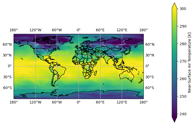
In this section, you’ll find quick instructions on how to reproject a dataset to a named projection. We’ll start by loading a sample dataset on a global regular latitude-longitude grid. The dataset is opened with Xarray, and we select the first time step, which will then be reprojected.
[3]:
import pyku.resources as resources
ds = resources.get_test_data('global_data').isel(time=0)
[4]:
ds.ana.one_map(var='tas')
<Figure size 640x480 with 0 Axes>
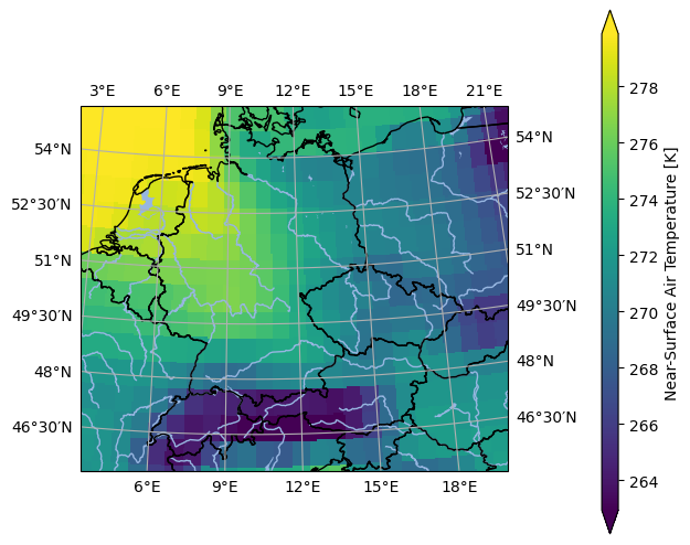
Since the HYR-LAEA-5 projection is predefined in pyku, we can import and reproject the data onto that grid with a single command.
[5]:
import pyku
projected = ds.pyku.project('HYR-LAEA-5')
You can then visualize the result as follows:
[6]:
projected.ana.one_map(
    var='tas',
    crs='HYR-LAEA-5',
    size_inches=(5, 5)
)
<Figure size 640x480 with 0 Axes>
As an aside, note that the data projection does not need to match the plot projection, which is defined using the crs parameter.
[7]:
projected.ana.one_map(
    var='tas',
    crs='EUR-44',
    size_inches=(5, 5)
)
<Figure size 640x480 with 0 Axes>

Most importantly, when projections are properly defined and maintained, all projection information is automatically embedded in the dataset. However, it’s worth noting that this involves substantial effort and ongoing work, and it typically requires a team rather than being a one-person task.
[8]:
projected.crs.attrs
[8]:
{'grid_mapping_name': 'lambert_azimuthal_equal_area',
 'longitude_of_projection_origin': 10.0,
 'latitude_of_projection_origin': 52.0,
 'semi_major_axis': 6378137.0,
 'semi_minor_axis': 6356752.31414036,
 'inverse_flattening': 298.257222101,
 'false_easting': 4321000.0,
 'false_northing': 3210000.0,
 'spatial_ref': 'PROJCS["ETRS_1989_LAEA",GEOGCS["GCS_ETRS_1989",DATUM["D_ETRS_1989",SPHEROID["GRS_1980",6378137.0,298.257222101]],PRIMEM["Greenwich",0.0],UNIT["Degree",0.0174532925199433]],PROJECTION["Lambert_Azimuthal_Equal_Area"],PARAMETER["False_Easting",4321000.0],PARAMETER["False_Northing",3210000.0],PARAMETER["Central_Meridian",10.0],PARAMETER["Latitude_Of_Origin",52.0],UNIT["Meter",1.0]]',
 'crs_wkt': 'PROJCS["ETRS_1989_LAEA",GEOGCS["GCS_ETRS_1989",DATUM["D_ETRS_1989",SPHEROID["GRS_1980",6378137.0,298.257222101]],PRIMEM["Greenwich",0.0],UNIT["Degree",0.0174532925199433]],PROJECTION["Lambert_Azimuthal_Equal_Area"],PARAMETER["False_Easting",4321000.0],PARAMETER["False_Northing",3210000.0],PARAMETER["Central_Meridian",10.0],PARAMETER["Latitude_Of_Origin",52.0],UNIT["Meter",1.0]]',
 'proj4': '+proj=laea +lat_0=52 +lon_0=10 +x_0=4321000 +y_0=3210000 +ellps=GRS80 +towgs84=0,0,0,0,0,0,0 +units=m +no_defs +type=crs',
 'proj4_params': '+proj=laea +lat_0=52 +lon_0=10 +x_0=4321000 +y_0=3210000 +ellps=GRS80 +towgs84=0,0,0,0,0,0,0 +units=m +no_defs +type=crs',
 'epsg_code': 'EPSG:3035',
 'long_name': 'DWD HYRAS ETRS89 LAEA grid with 258 columns and 220 rows'}
Named projections#
You can obtain the full list of default projections included in pyku using the following command:
[9]:
import pyku.geo as geo
geo.list_standard_areas()
[9]:
['EUR-44',
 'EUR-11',
 'EUR-6',
 'GER-0275',
 'EPISODES',
 'radolan_wx',
 'DWD_RADOLAN_1100x900',
 'DWD_RADOLAN_900x900',
 'HOSTRADA-1',
 'linet_eqc',
 'euradcom_ps',
 'euradcom_eqc',
 'world_360x180',
 'world_540x270',
 'world_7200x3600',
 'world_3600x1800',
 'world_43200x21600',
 'seamless_europe',
 'seamless_world',
 'seamless_germany',
 'HYR-LCC-1',
 'HYR-LCC-3',
 'HYR-LCC-5',
 'HYR-LCC-125',
 'HYR-LCC-50',
 'HYR-LAEA-1',
 'HYR-LAEA-2',
 'HYR-LAEA-3',
 'HYR-LAEA-5',
 'HYR-LAEA-12.5',
 'HYR-LAEA-50',
 'HYR-LAEA-100',
 'HYR-GER-LAEA-1',
 'HYR-GER-LAEA-2',
 'HYR-GER-LAEA-3',
 'HYR-GER-LAEA-5',
 'HYR-GER-LAEA-12.5',
 'HYR-GER-LAEA-50',
 'HYR-GER-LAEA-100',
 'cerra']
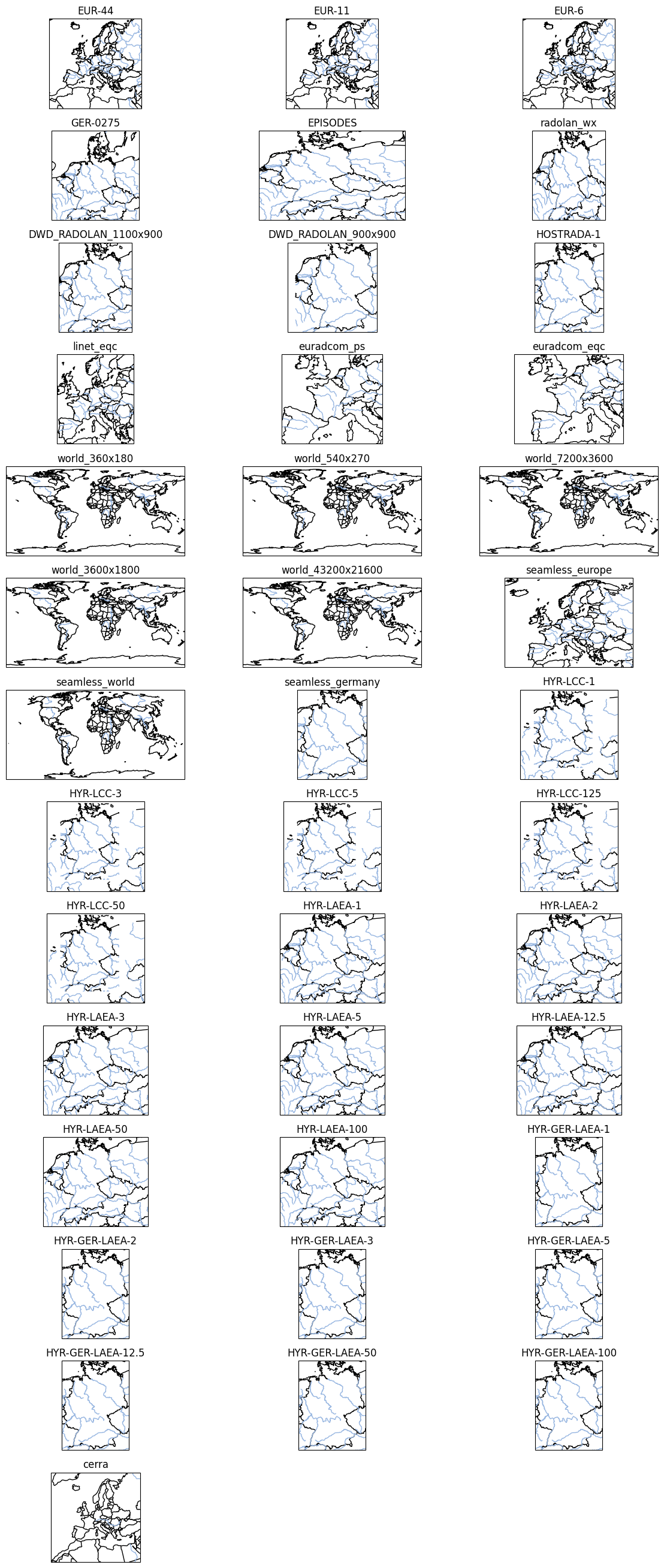
The following code allows you to visualize all named projections included in pyku:
[10]:
import matplotlib.pyplot as plt
import cartopy
import cartopy.feature
import pyku.geo as geo
from matplotlib.gridspec import GridSpec

area_names = list(geo.get_areas_definitions().keys())
nrows = len(area_names) // 3 + (len(area_names) % 3) * 3

fig = plt.figure(figsize=(12, 30))
gs = GridSpec(nrows, 3, figure=fig)

for idx, area_name in enumerate(area_names):
    pyresample_crs = geo.load_area_def(area_name)
    cartopy_crs = pyresample_crs.to_cartopy_crs()
    ax = fig.add_subplot(gs[idx], projection=cartopy_crs)
    ax.set_title(area_name)
    ax.add_feature(cartopy.feature.COASTLINE)
    ax.add_feature(cartopy.feature.BORDERS)
    ax.add_feature(cartopy.feature.RIVERS)

fig.tight_layout()
Parameters and formats#
The following section demonstrates how to obtain pyresample AreaDefinition objects or a Cartopy CRS. It also shows and discusses how to retrieve projection strings, WKT strings, EPSG codes, and CF-compliant projection definitions.
pyresample AreaDefinition#
The default object dealing with projections in pyku is the pyresample.AreaDefinition object from the PyTROLL project. Parameters can obtained directly from the dataset and shown with:
[11]:
projected = ds.pyku.project('HYR-LAEA-5')
area_def = projected.pyku.get_area_def()
area_def
[11]:
Area ID: crs
Description: crs
Projection: {'ellps': 'GRS80', 'lat_0': '52', 'lon_0': '10', 'no_defs': 'None', 'proj': 'laea', 'type': 'crs', 'units': 'm', 'x_0': '4321000', 'y_0': '3210000'}
Number of columns: 258
Number of rows: 220
Area extent: (3806000.0, 2489000.0, 5096000.0, 3589000.0)
Cartopy coordinate reference system#
You can obtain a Cartopy CRS with the following command and use it directly for plotting with Cartopy.
[12]:
area_def = projected.pyku.get_area_def()
area_def.to_cartopy_crs()
[12]:
<pyresample.utils.cartopy.Projection object at 0x7f4850300d40>
PROJ string#
In the same manner, you can obtain the proj string:
[13]:
area_def = projected.pyku.get_area_def()
area_def.proj_str
[13]:
'+ellps=GRS80 +lat_0=52 +lon_0=10 +no_defs +proj=laea +type=crs +units=m +x_0=4321000 +y_0=3210000'
WKT string#
In the same manner, you can obtain the proj string:
[14]:
area_def = projected.pyku.get_area_def()
area_def.crs_wkt
[14]:
'PROJCRS["ETRS89-extended / LAEA Europe",BASEGEOGCRS["ETRS89",DATUM["European Terrestrial Reference System 1989",ELLIPSOID["GRS 1980",6378137,298.257222101,LENGTHUNIT["metre",1]],ID["EPSG",6258]],PRIMEM["Greenwich",0,ANGLEUNIT["Degree",0.0174532925199433]]],CONVERSION["unnamed",METHOD["Lambert Azimuthal Equal Area",ID["EPSG",9820]],PARAMETER["Latitude of natural origin",52,ANGLEUNIT["Degree",0.0174532925199433],ID["EPSG",8801]],PARAMETER["Longitude of natural origin",10,ANGLEUNIT["Degree",0.0174532925199433],ID["EPSG",8802]],PARAMETER["False easting",4321000,LENGTHUNIT["metre",1],ID["EPSG",8806]],PARAMETER["False northing",3210000,LENGTHUNIT["metre",1],ID["EPSG",8807]]],CS[Cartesian,2],AXIS["(E)",east,ORDER[1],LENGTHUNIT["metre",1,ID["EPSG",9001]]],AXIS["(N)",north,ORDER[2],LENGTHUNIT["metre",1,ID["EPSG",9001]]]]'
CF-conform area definition#
If available, the CF-conform area definition can be read directly from the attributes of the crs variable
[15]:
area_def = projected.pyku.get_area_def()
projected.crs.attrs
[15]:
{'grid_mapping_name': 'lambert_azimuthal_equal_area',
 'longitude_of_projection_origin': 10.0,
 'latitude_of_projection_origin': 52.0,
 'semi_major_axis': 6378137.0,
 'semi_minor_axis': 6356752.31414036,
 'inverse_flattening': 298.257222101,
 'false_easting': 4321000.0,
 'false_northing': 3210000.0,
 'spatial_ref': 'PROJCS["ETRS_1989_LAEA",GEOGCS["GCS_ETRS_1989",DATUM["D_ETRS_1989",SPHEROID["GRS_1980",6378137.0,298.257222101]],PRIMEM["Greenwich",0.0],UNIT["Degree",0.0174532925199433]],PROJECTION["Lambert_Azimuthal_Equal_Area"],PARAMETER["False_Easting",4321000.0],PARAMETER["False_Northing",3210000.0],PARAMETER["Central_Meridian",10.0],PARAMETER["Latitude_Of_Origin",52.0],UNIT["Meter",1.0]]',
 'crs_wkt': 'PROJCS["ETRS_1989_LAEA",GEOGCS["GCS_ETRS_1989",DATUM["D_ETRS_1989",SPHEROID["GRS_1980",6378137.0,298.257222101]],PRIMEM["Greenwich",0.0],UNIT["Degree",0.0174532925199433]],PROJECTION["Lambert_Azimuthal_Equal_Area"],PARAMETER["False_Easting",4321000.0],PARAMETER["False_Northing",3210000.0],PARAMETER["Central_Meridian",10.0],PARAMETER["Latitude_Of_Origin",52.0],UNIT["Meter",1.0]]',
 'proj4': '+proj=laea +lat_0=52 +lon_0=10 +x_0=4321000 +y_0=3210000 +ellps=GRS80 +towgs84=0,0,0,0,0,0,0 +units=m +no_defs +type=crs',
 'proj4_params': '+proj=laea +lat_0=52 +lon_0=10 +x_0=4321000 +y_0=3210000 +ellps=GRS80 +towgs84=0,0,0,0,0,0,0 +units=m +no_defs +type=crs',
 'epsg_code': 'EPSG:3035',
 'long_name': 'DWD HYRAS ETRS89 LAEA grid with 258 columns and 220 rows'}
Custom projection definition#
pyku named area definitions are stored in the areas.yaml file distributed with the library, while CF-compliant metadata is found in the areas_cf.yaml file. Defining and maintaining these configurations is a complex task, and contributions or assistance are greatly appreciated. The following section details the internal workings of pyku related to constructing and integrating new grids. Note that any arbitrary projection can be created and used in pyku in this manner, though it
requires a deep understanding of the underlying complexities.
External documentation#
Projecting uses pyresample/PROJ in the background:
Internal format#
Prepared named area definitions follow the PyTROLL format, based on the PROJ library, and are structured as follows:
linet_eqc:
  description: Linet coverage with a 3000 meters SSP resolution
  projection:
    proj: eqc
    lat_ts: 50.0
    lon_0: 10.0
    a: 6378137.0
    b: 6356752.3142
    h: 35785863.0
  shape:
    height: 1114
    width: 956
  area_extent:
    lower_left_xy: [-1431096.0, 3896182.0]
    upper_right_xy: [1431096.0, 7235767.0]

world_3600x1800:
  description: World image
  projection:
    proj: eqc
    lon_0: 0.0
    a: 6378137.0
    b: 6356752.3142
  shape:
    height: 1800
    width: 3600
  area_extent:
    lower_left_xy: [-20037508.34, -10018754.17]
    upper_right_xy: [20037508.34, 10018754.17]
Example: RADOLAN projection#
First you need to define the lower left and upper right corner in projection cooordinates:
[16]:
import pyproj

# Geographic coordinates of lower lef (ll) and upper right (ur) corners
# ---------------------------------------------------------------------

lat_ll = 46.9526
lon_ll =  3.5889
lat_ur = 54.7405
lon_ur = 15.7208

# The proj string can be taken from wradlib
# -----------------------------------------

proj_string = '+proj=stere +lat_0=90 +lat_ts=60 +lon_0=10 \
+x_0=0 +y_0=0 +R=6370040 +units=km +no_defs'

# Source projection are the geographic coordinates on a WGS84 earth
# -----------------------------------------------------------------

transformer = pyproj.Transformer.from_crs(
    'EPSG:4326',
    proj_string,
    always_xy=True
)

# Transform geographic coordinates to projection coordinates
# ----------------------------------------------------------

x_ll, y_ll = transformer.transform(lon_ll, lat_ll)
x_ur, y_ur = transformer.transform(lon_ur, lat_ur)

x_ll, y_ll = round(x_ll, 4), round(y_ll, 4)
x_ur, y_ur = round(x_ur, 4), round(y_ur, 4)

lower_left_x, lower_left_y, upper_right_x, upper_right_y = \
    x_ll, y_ll, x_ur, y_ur

lower_left_x, lower_left_y, upper_right_x, upper_right_y
[16]:
(-523.4643, -4658.6421, 376.5413, -3758.6499)
Now that the area extent has been calculated, we can create an area definition that can be included in pyku.
[17]:
import pyproj
from pyresample.geometry import AreaDefinition
area_id = 'DWD_RADOLAN_900x900'
description = 'DWD RADOLAN projection'
proj_id = 'dwd_radolan'
projection = proj_string
width = 900
height = 900
area_extent =  (lower_left_x, lower_left_y, upper_right_x, upper_right_y)

area_def = AreaDefinition(
    area_id,
    description,
    proj_id,
    projection,
    width,
    height,
    area_extent
)

print(area_def.dump())
DWD_RADOLAN_900x900:
  description: DWD RADOLAN projection
  projection:
    proj: stere
    lat_0: 90
    lat_ts: 60
    lon_0: 10
    x_0: 0
    y_0: 0
    R: 6370040
    no_defs: null
    type: crs
  shape:
    height: 900
    width: 900
  area_extent:
    lower_left_xy: [-523.4643, -4658.6421]
    upper_right_xy: [376.5413, -3758.6499]
    units: km
Example an equirectangular projection#
The following script generates the input to create an equirectangular projection covering the entire world. Adjust the latitude and longitude values as needed. Copy the code into a file named myprojection.py and run it.
[18]:
# Import the pyproj libraries
# ---------------------------

import pyproj

# Define the proj string
# ----------------------

proj_string = '+proj=eqc +lat_ts=0.0 +lat_0=0.0 +lon_0=0.0 +a=6378137.0 +b=6356752.3'

# The source projection are the geographic coordinates on a WGS84 earth
# ---------------------------------------------------------------------

wgs84_latlong_proj = pyproj.Proj(proj='latlong', datum='WGS84')

# Create transformer and transform
# ------------------

transformer = pyproj.Transformer.from_proj(
    proj_from=wgs84_latlong_proj, proj_to=proj_string
)

x_ll, y_ll = transformer.transform(lon_ll, lat_ll)
x_ur, y_ur = transformer.transform(lon_ur, lat_ur)

x_ll, y_ll = round(x_ll, 4), round(y_ll, 4)
x_ur, y_ur = round(x_ur, 4), round(y_ur, 4)

lower_left_x, lower_left_y, upper_right_x, upper_right_y = x_ll, y_ll, x_ur, y_ur

# Set the number of pixels in the x and y direction
# -------------------------------------------------

x_size=7200
y_size=3200

from pyresample.geometry import AreaDefinition
area_id = 'world_eqc'
description = 'World regular lat lon'
proj_id = 'world_eqc'
projection = proj_string
width = x_size
height = y_size
area_extent =  (lower_left_x, lower_left_y, upper_right_x, upper_right_y)

area_def = AreaDefinition(
    area_id,
    description,
    proj_id,
    projection,
    width,
    height,
    area_extent
)

print(area_def.dump())
world_eqc:
  description: World regular lat lon
  projection:
    proj: eqc
    lat_ts: 0
    lat_0: 0
    lon_0: 0
    x_0: 0
    y_0: 0
    a: 6378137
    rf: 298.257024882273
    no_defs: null
    type: crs
  shape:
    height: 3200
    width: 7200
  area_extent:
    lower_left_xy: [399514.5205, 5226739.5234]
    upper_right_xy: [1750031.4509, 6093684.5858]
    units: m
Geodetic parameters#
Geodetic paramers can be taken from the following references:
National Imagery and Mapping Agency (NIMA), Department of Defense World Geodetic System 1984, NIMA TR8350.2, third edition, 2000
Equator radius: 6378137.0 meters
Polar radius: 6356752.3142 meters
Inverse flattening: 298.257223563
EUMETSAT, LRIT/HRIT Global Specifications, CGMS/DOC/12/0017, issue 2.8, 2013 par 4.4.3.2
Distance between spacecraft and the radius of the earth: 42164 km
Equator radius: 6378.1370 km
Polar radius: 6356.7523 km
Altitude of the spacecraft: 35785.863 km
Constant:
\(\pi\)/180 0.017453292519943295