
Polygons#
Import resources#
[1]:
import pyku
import pyku.resources as resources
import pyku.analyse as analyse
Download directory#
Polygons are mostly downloaded on-the-fly. The download takes place only one time and the downloaded data are reused if the polygons are called twice. The download path can be shown with. If you set the environment variable PYKU_DATA_DIR, the data will automatically be downloaded in that directory. If you do not set that environment variable, data are downloaded by default in the standard directory ~/.local/share/pyku. You can also overwrite the data_dir during runtime using
pyku.PYKU_CONFIG.set(data_dir) = <your_new_data_dir>, but there wont be any sanity checks that way, so the directory needs to exist and needs to have the right permissions set.
[2]:
pyku.PYKU_CONFIG
[2]:
<pyku.core.config_provider.PykuConfigProvider at 0x7f47e23fb8c0>
List of available polygons#
The identifier of all available polygons can be accessed like so:
[3]:
resources.list_polygon_identifiers()
[3]:
['ne_10m_admin_0_countries',
 'ne_10m_coastline',
 'ne_10m_rivers',
 'ne_10m_lakes',
 'germany',
 'austria',
 'german_states',
 'german_cities',
 'ne_10m_geography_regions_polys',
 'eobs_mask',
 'prudence',
 'natural_areas_of_germany',
 'natural_areas_of_germany_merged4',
 'german_directions',
 'natural_climatic_regions_of_germany']
Germany#
[4]:
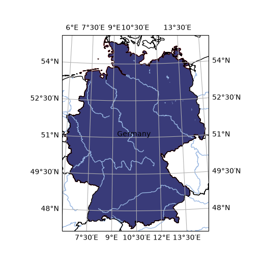
geodf = resources.get_geodataframe('germany')

print(f"{resources.pyku_resources.get('polygons').get('germany').get('description')}")

analyse.regions(
    geodf,
    area_def='HYR-GER-LAEA-5',
    size_inches=(5, 5)
)
Germany selected from https://www.naturalearthdata.com/downloads/10m-cultural-vectors/10m-admin-0-countries/
German cities#
[5]:
# Get German cities
# -----------------

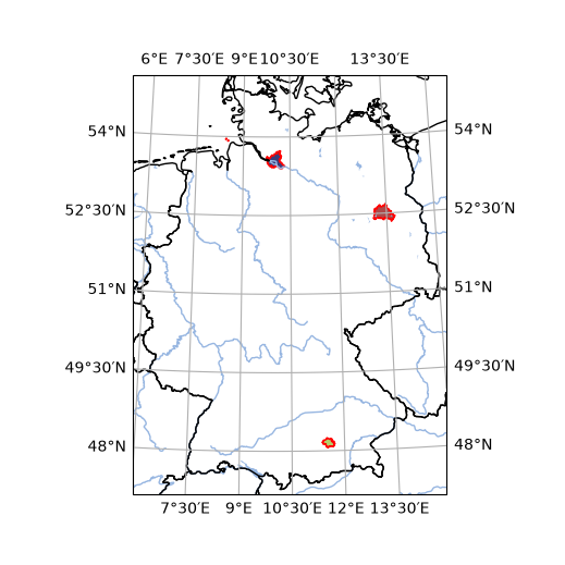
geodf = resources.get_geodataframe('german_cities')

# Get description
# ---------------

print(f"{resources.pyku_resources.get('polygons').get('german_cities').get('description')}")

# Select 'Kreisfreie Stadt'
# -------------------------

geodf = geodf.query("BEZ == 'Kreisfreie Stadt'")

# Select cities
# -------------

geodf = geodf[geodf['GEN'].isin(['Frankfurt', 'Offenbach', 'Berlin', 'Hamburg', 'München'])]

# Plot
# ----

analyse.regions(
    geodf,
    area_def='HYR-GER-LAEA-5',
    size_inches=(5, 5)
)
Downloading file 'vg250_01-01.tm32.shape.ebenen.zip' from 'https://daten.gdz.bkg.bund.de/produkte/vg/vg250_ebenen_0101/aktuell/vg250_01-01.tm32.shape.ebenen.zip' to '/home/runner/work/pyku/pyku/pyku_cache'.
Unzipping contents of '/home/runner/work/pyku/pyku/pyku_cache/vg250_01-01.tm32.shape.ebenen.zip' to '/home/runner/work/pyku/pyku/pyku_cache/vg250_01-01.tm32.shape.ebenen.zip.unzip'
See https://gdz.bkg.bund.de/index.php/default/digitale-geodaten/verwaltungsgebiete/verwaltungsgebiete-1-250-000-stand-01-01-vg250-01-01.html
The alps#
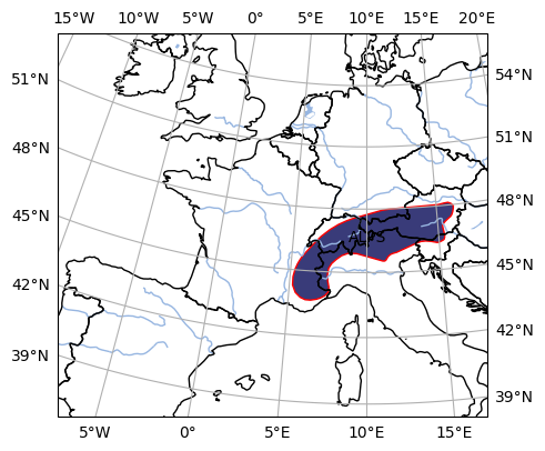
Load regions with
[6]:
geodf = resources.get_geodataframe('ne_10m_geography_regions_polys')
Downloading file 'ne_10m_geography_regions_polys.zip' from 'https://naturalearth.s3.amazonaws.com/10m_physical/ne_10m_geography_regions_polys.zip' to '/home/runner/work/pyku/pyku/pyku_cache'.
Unzipping contents of '/home/runner/work/pyku/pyku/pyku_cache/ne_10m_geography_regions_polys.zip' to '/home/runner/work/pyku/pyku/pyku_cache/ne_10m_geography_regions_polys.zip.unzip'
Search any rows that would contain the word alps
[7]:
rows = (geodf.map(lambda x: str(x).lower() == 'alps')).any(axis=1)
geodf.loc[rows]
[7]:
| FEATURECLA | NAME | NAMEALT | REGION | SUBREGION | MIN_LABEL | MAX_LABEL | SCALERANK | LABEL | WIKIDATAID | ... | NAME_TR | NAME_VI | NAME_ZH | NE_ID | NAME_FA | NAME_HE | NAME_UK | NAME_UR | NAME_ZHT | geometry | |
|---|---|---|---|---|---|---|---|---|---|---|---|---|---|---|---|---|---|---|---|---|---|
| 712 | Range/mtn | ALPS | NaN | Europe | NaN | 2.0 | 8.0 | 1 | ALPS | Q1286 | ... | Alpler | Anpơ | 阿尔卑斯山 | 1159104297 | آلپ | הרי האלפים | Альпи | الپس | 阿尔卑斯山 | POLYGON ((15.31483 46.43159, 15.26673 46.40217... |
1 rows × 38 columns
[8]:
# Get the Alps
# ------------

geodf = geodf.query("NAME == 'ALPS'")

# Plot
# ----

analyse.regions(
    geodf,
    area_def='euradcom_ps',
    size_inches=(5, 5)
)
Natural areas of Germany#
[9]:
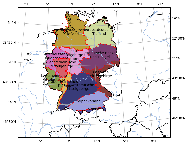
geodf = resources.get_geodataframe('natural_areas_of_germany')

# Plot
# ----

analyse.regions(
    geodf,
    area_def='HYR-LAEA-5',
    size_inches=(8, 8),
)
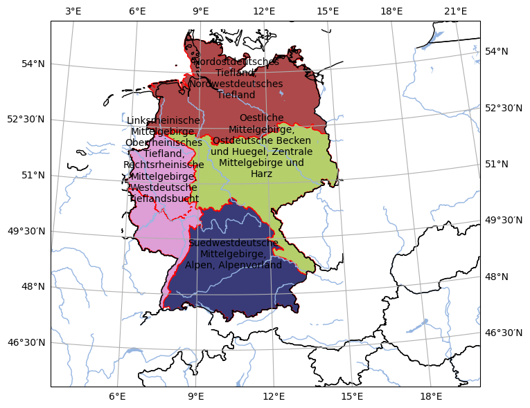
The merged polygons can be accessed with:
[10]:
geodf = resources.get_geodataframe('natural_areas_of_germany_merged4')

display(geodf)

# Plot
# ----

analyse.regions(
    geodf,
    area_def='HYR-LAEA-5',
    size_inches=(8, 8),
)
| index | geometry | NAME | DIRECTION | |
|---|---|---|---|---|
| 0 | 0 | POLYGON ((3620123.5 5271088, 3620109 5270726, ... | Suedwestdeutsche Mittelgebirge, Alpen, Alpenvo... | South |
| 1 | 0 | POLYGON ((3920531.75 5696475, 3920604.5 569651... | Oestliche Mittelgebirge, Ostdeutsche Becken un... | East |
| 2 | 0 | MULTIPOLYGON (((3786207 6069685, 3786176.5 606... | Nordostdeutsches Tiefland, Nordwestdeutsches T... | North |
| 3 | 0 | POLYGON ((3496914.5 5596087, 3496785 5596087, ... | Linksrheinische Mittelgebirge, Oberrheinisches... | West |
Climatic Natural Regions of Germany#
[11]:
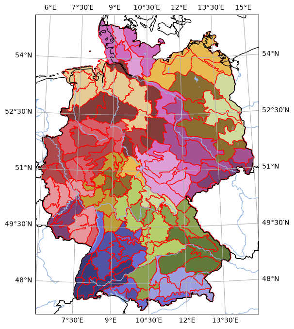
geodf = resources.get_geodataframe('natural_climatic_regions_of_germany')

display(geodf)

# Plot
# ----

analyse.regions(
    geodf,
    area_def='HYR-GER-LAEA-5',
    size_inches=(8, 8),
)
| KLINATID | ORD3 | NAME_ORD3 | FLÄCHE | HAUPTEINHEIT | KATEGORIE | BUNDESLAND | REGIONSID | geometry | |
|---|---|---|---|---|---|---|---|---|---|
| 0 | 1 | 160, 90, 161, 160 | Hochrheintal, Randen (Klettgau- u. Randenalb),... | 339.722550 | 443, 445, 446, 447 | rot | Baden-Württemberg | BW_001 | MULTIPOLYGON (((8.45979 47.59533, 8.45992 47.5... |
| 1 | 2 | 154, 155 | Südöstlicher Schwarzwald, Hochschwarzwald | 2074.765855 | 417, 424 | grün | Baden-Württemberg | BW_002 | MULTIPOLYGON (((8.19638 47.69281, 8.18063 47.6... |
| 2 | 3 | 201, 202, 203, 200 | Markgräfler Hügelland, Freiburger Bucht, Kaise... | 887.246683 | 427, 420, 418, 419 | grün | Baden-Württemberg | BW_003 | MULTIPOLYGON (((7.72307 47.86668, 7.71966 47.8... |
| 3 | 4 | 93, 92, 121, 120 | Hohe Schwabenalb, Baaralb und Oberes Donautal,... | 1877.069162 | 421, 415, 409, 432 | grün | Baden-Württemberg | BW_004 | MULTIPOLYGON (((8.5369 47.80537, 8.53859 47.79... |
| 4 | 5 | 95, 40, 90, 91, 90 | Mittlere Flächenalb, Donau-Ablach-Platten, Ran... | 2445.904271 | 433, 436, 422, 412, 401 | grün | Baden-Württemberg | BW_005 | MULTIPOLYGON (((8.57036 47.80623, 8.57001 47.8... |
| ... | ... | ... | ... | ... | ... | ... | ... | ... | ... |
| 143 | 144 | 391, 390, 392, 393 | Thüringer Wald, Südliches Vorland des Thüringe... | 3925.504688 | 507, 244, 282, 259 | grün | Thüringen, Bayern | BY-TH_144 | MULTIPOLYGON (((12.01365 50.28808, 12.03116 50... |
| 144 | 145 | 483, 373, 375 | Ringgau, Hainich, Obereichsfeld, Dün-Hainleite... | 1971.729628 | 171, 181, 195 | grün | Thüringen, Niedersachsen, Hessen | HE-NI-TH_145 | MULTIPOLYGON (((10.56891 51.40376, 10.58622 51... |
| 145 | 146 | 410, 411 | Ostthüringisch-Vogtländische Hochflächen, Mitt... | 2369.840132 | 253, 229 | grün | Thüringen, Sachsen, Bayern | BY-SN-TH_146 | MULTIPOLYGON (((12.32822 50.6997, 12.31361 50.... |
| 146 | 147 | 472, 471, 470 | Mittleres Saaletal, Saale-Elster-Sandsteinplat... | 1296.993201 | 223, 248, 217 | orange | Thüringen, Sachsen-Anhalt | ST-TH_147 | MULTIPOLYGON (((11.30151 50.71812, 11.32294 50... |
| 147 | 148 | 487, 489, 488, 482 | Helme-Unstrut-Niederung, Querfurter Platte und... | 4348.115359 | 182, 180, 179, 505 | grün | Thüringen, Sachsen-Anhalt | ST-TH_148 | MULTIPOLYGON (((11.59763 51.06798, 11.58592 51... |
148 rows × 9 columns
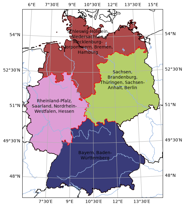
Germany split into western, northern, easter and south Germany#
[12]:
geodf = resources.get_geodataframe('german_directions')

# Plot
# ----

analyse.regions(
    geodf,
    area_def='HYR-GER-LAEA-5',
    size_inches=(8, 8),
)
Downloading file 'ne_10m_admin_1_states_provinces.zip' from 'https://naturalearth.s3.amazonaws.com/10m_cultural/ne_10m_admin_1_states_provinces.zip' to '/home/runner/work/pyku/pyku/pyku_cache'.
Unzipping contents of '/home/runner/work/pyku/pyku/pyku_cache/ne_10m_admin_1_states_provinces.zip' to '/home/runner/work/pyku/pyku/pyku_cache/ne_10m_admin_1_states_provinces.zip.unzip'
German states#
[13]:
geodf = resources.get_geodataframe('german_states')

analyse.regions(
    geodf,
    area_def='HYR-GER-LAEA-5',
    size_inches=(8, 8),
)
World#
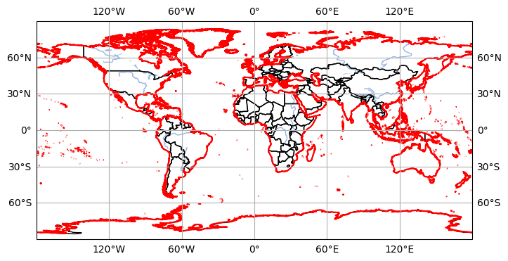
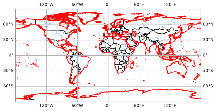
Polygons for the whole world is quite easy.
[14]:
geodf = resources.get_geodataframe('ne_10m_coastline')

analyse.regions(
    geodf,
    area_def='world_360x180',
    size_inches=(8, 8),
)
Downloading file 'ne_10m_coastline.zip' from 'https://naturalearth.s3.amazonaws.com/10m_physical/ne_10m_coastline.zip' to '/home/runner/work/pyku/pyku/pyku_cache'.
Unzipping contents of '/home/runner/work/pyku/pyku/pyku_cache/ne_10m_coastline.zip' to '/home/runner/work/pyku/pyku/pyku_cache/ne_10m_coastline.zip.unzip'
Configuration file#
The data are configured per yaml file. Users do not need to worry about it unless new polygons are needed. The source of the data is available in the description. You can get the configuration as a python dictionary like so
[15]:
import pyku.resources as resources
resources.pyku_resources
[15]:
{'polygons': {'ne_10m_admin_0_countries': {'description': 'See https://www.naturalearthdata.com/downloads/10m-cultural-vectors/10m-admin-0-countries/\n',
   'base_url': 'https://naturalearth.s3.amazonaws.com/10m_cultural/',
   'archive_file': 'ne_10m_admin_0_countries.zip',
   'target_file': 'ne_10m_admin_0_countries.shp',
   'query': None,
   'aliases': ['countries']},
  'ne_10m_coastline': {'description': 'See https://www.naturalearthdata.com/downloads/10m_physical/ne_10m_coastline/\n',
   'base_url': 'https://naturalearth.s3.amazonaws.com/10m_physical/',
   'archive_file': 'ne_10m_coastline.zip',
   'target_file': 'ne_10m_coastline.shp',
   'query': None},
  'ne_10m_rivers': {'description': 'See https://www.naturalearthdata.com/downloads/10m-physical-vectors/10m-rivers-lake-centerlines/\n',
   'base_url': 'https://naturalearth.s3.amazonaws.com/10m_physical/',
   'archive_file': 'ne_10m_rivers_lake_centerlines.zip',
   'target_file': 'ne_10m_rivers_lake_centerlines.shp',
   'query': None},
  'ne_10m_lakes': {'description': 'See https://www.naturalearthdata.com/downloads/10m-physical-vectors/10m-lakes/\n',
   'base_url': 'https://naturalearth.s3.amazonaws.com/10m_physical/',
   'archive_file': 'ne_10m_lakes.zip',
   'target_file': 'ne_10m_lakes.shp',
   'query': None},
  'germany': {'description': 'Germany selected from https://www.naturalearthdata.com/downloads/10m-cultural-vectors/10m-admin-0-countries/\n',
   'base_url': 'https://naturalearth.s3.amazonaws.com/10m_cultural/',
   'archive_file': 'ne_10m_admin_0_countries.zip',
   'target_file': 'ne_10m_admin_0_countries.shp',
   'query': "SOVEREIGNT == 'Germany'"},
  'austria': {'description': 'Austria selected from https://www.naturalearthdata.com/downloads/10m-cultural-vectors/10m-admin-0-countries/\n',
   'base_url': 'https://naturalearth.s3.amazonaws.com/10m_cultural/',
   'archive_file': 'ne_10m_admin_0_countries.zip',
   'target_file': 'ne_10m_admin_0_countries.shp',
   'query': "SOVEREIGNT == 'Austria'"},
  'german_states': {'description': 'German states selected from https://www.naturalearthdata.com/downloads/10m-cultural-vectors/10m-admin-1-states-provinces/\n',
   'base_url': 'https://naturalearth.s3.amazonaws.com/10m_cultural/',
   'archive_file': 'ne_10m_admin_1_states_provinces.zip',
   'target_file': 'ne_10m_admin_1_states_provinces.shp',
   'query': "iso_a2 == 'DE'"},
  'german_cities': {'description': 'See https://gdz.bkg.bund.de/index.php/default/digitale-geodaten/verwaltungsgebiete/verwaltungsgebiete-1-250-000-stand-01-01-vg250-01-01.html\n',
   'base_url': 'https://daten.gdz.bkg.bund.de/produkte/vg/vg250_ebenen_0101/aktuell/',
   'archive_file': 'vg250_01-01.tm32.shape.ebenen.zip',
   'target_file': 'VG250_KRS.shp',
   'query': None},
  'ne_10m_geography_regions_polys': {'description': 'See https://www.naturalearthdata.com/downloads/10m-physical-vectors/10m-physical-labels/\n',
   'base_url': 'https://naturalearth.s3.amazonaws.com/10m_physical/',
   'archive_file': 'ne_10m_geography_regions_polys.zip',
   'target_file': 'ne_10m_geography_regions_polys.shp',
   'query': None,
   'aliases': ['geographic_regions']},
  'eobs_mask': {'description': '\nMask for the usage of E-OBS data in anlyses like pyku.ana.mean_vs_time. It was generated using E-OBS v27.0 ensemble mean data at 0.1 deg resolution. It is the minimum overlap of valid data of all available variables, averaged over the year 1979.\nREFERENCES\n* https://www.ecad.eu/download/ensembles/download.php *  Cornes, R. C., van der Schrier, G., van den Besselaar, E. J. M., & Jones, P. D. (2018).\n   An ensemble version of the E-OBS temperature and precipitation data sets.\n   JGR: Atmospheres, 123, 9391-9409. https://doi.org/10.1029/2017JD028200\n',
   'base_url': None,
   'archive_file': None,
   'target_file': 'eobs_mask.geojson.zip',
   'query': None},
  'prudence': {'description': '\nPrudence polygons, used in climatology, are spatial divisions developed during the PRUDENCE project (Prediction of Regional scenarios and Uncertainties for Defining EuropeaN Climate change risks and Effects). These polygons are defined to represent consistent and climatically homogeneous regions across Europe, facilitating regional climate change analyses. They are widely used for studying the impacts of climate models at sub-continental scales and are essential for evaluating regional climate projections under various scenarios. The polygons provide a framework for aggregating climate model data, aiding in the comparison of regional impacts under different climate conditions. These regions correspond to specific areas that experience similar climatic patterns and help in better understanding variability and extreme events under modeled and observed datasets.\nREFERENCES\n* https://ensemblesrt3.dmi.dk/quicklook/regions.html * https://www.wcrp-climate.org/modelling-wgcm-mip-catalogue/modelling-wgcm-mips-2/288-modelling-wgcm-catalogue-prudence * Christensen, J.H., Christensen, O.B. A summary of the PRUDENCE model\n  projections of changes in European climate by the end of this century.\n  Climatic Change 81 (Suppl 1), 7-30 (2007).\n  https://doi.org/10.1007/s10584-006-9210-7\n',
   'base_url': None,
   'archive_file': None,
   'target_file': 'prudence.geojson.zip',
   'query': None},
  'natural_areas_of_germany': {'description': 'Not documented',
   'base_url': None,
   'archive_file': None,
   'target_file': 'Regionen_NationalerKlimareport_2015_Namen.geojson.zip',
   'query': None},
  'natural_areas_of_germany_merged4': {'description': 'Natural areas of Germany divided into western, northern, eastern and southern states.\nWestern  - Linksrheinische Mittelgebirge, Oberrheinisches Tiefland,\n           Rechtsrheinische Mittelgebirge, Westdeutsche Tieflandsbucht\nNorthern - Nordostdeutsches Tiefland, Nordwestdeutsches Tiefland Eastern  - Oestliche Mittelgebirge, Ostdeutsche Becken und Huegel,\n           Zentrale Mittelgebirge und Harz\nSouthern - Suedwestdeutsche Mittelgebirge, Alpen, Alpenvorland\nThese polygons are built on-the-fly from Natural Areas of Germany data available in pyku. See the source code in resources.py\n',
   'base_url': None,
   'archive_file': None,
   'target_file': None,
   'query': None},
  'german_directions': {'description': "Germany divided into western, northern, eastern and southern states.\nWestern states  - Rheinland-Pfalz, Saarland, Nordrhein-Westfalen,\n                  Hessen,\nNorthern states - Schleswig-Holstein, Hamburg, Bremen, Niedersachsen,\n                  Mecklenburg-Vorpommern'\nEastern states  - Berlin, Brandenburg, Sachsen, Sachsen-Anhalt,\n                  Thüringen\nSouthern states - Bayern, Baden-Württemberg,\nThese polygons are built on-the-fly from German states data available in ne_10m_admin_1_states_provinces. See the source code in resources.py\n",
   'base_url': None,
   'archive_file': None,
   'target_file': None,
   'query': None},
  'natural_climatic_regions_of_germany': {'description': 'Natural climatic regions of Germany, as described in  https://www.dwd.de/DE/leistungen/klimaprojektionsdaten/pdf/naturraeume.html (German)\n',
   'base_url': 'https://github.com/deutscherwetterdienst/pyku-data/raw/main/geodata',
   'archive_file': 'KliNat-DWD.geojson.zip',
   'target_file': 'KliNat-DWD.geojson',
   'query': None}}}