Downscaling

This example shows how to perform downscaling with singular value decomposition

Time-dependent georeferenced data (e.g. temperature) are expressed as \(M\) matrices or size \(m \times n\) where \(m\) is the pixel index and \(n\) is the time index. Each weather situation is interpreted as a vector that can be decomposed in a basis of the vector space of possible weather situations. With singular valude decomposition (SVD), an orthonormal basis is calculated and ordered by how each basis vector is important. The basis is calculated for know observation weather data in low and high resolution.

Low resolution data from e.g. model calculation are projected to the low resolution observation data basis vectors, and brought up to high resolution by associating the known high resolution observation data basis vectors:

\[M_{\texttt{high-res-model}} = U_{\texttt{high-res-training}} U^T_{\texttt{low-res-training}} M_{\texttt{low-res-model}}\]

Where the \(U_{\texttt{low-res-training}}\) and \(U_{\texttt{high-res-training}}\) matrices contain the ordered basis vectors of high and low resolution observation/training data obtained by performing singular value decomposition.

Singular value decomposition

Any matrix \(M\) can be decomposed in the following way:

For real matrices, we have \(M^T=M^*\)

Decomposition of training data

\[\begin{split}\begin{align} M_{\texttt{low-res-training}} &= U_{\texttt{low-res-training}} \Sigma_{\texttt{low-res-training}} V^T_{\texttt{low-res-training}} \\ M_{\texttt{high-res-training}} & = U_{\texttt{high-res-training}} \Sigma_{\texttt{high-res-training}} V^T_{\texttt{high-res-training}} \\ \end{align}\end{split}\]

Basis vectors of the high resolution observation/training data

First forcing

High resolution and low resolution training data contain the same information, albeit at a difference resolution. The singular values \(\Sigma\) as well as associated covector matrices \(V\) are equal. This is forced by taking:

\[\begin{split}\begin{align} \Sigma_{\texttt{high-res-training}} &= \Sigma_{\texttt{low-res-training}} \\ V^T_{\texttt{high-res-training}} &= V^T_{\texttt{low-res-training}} \\ \end{align}\end{split}\]

With the forcing, we can replace:

\[M_{\texttt{high-res-training}} = U_{\texttt{high-res-training}} \Sigma_{\texttt{low-res-training}} V^T_{\texttt{low-res-training}}\]

And from there we can obtain the basis vectors both for high and low resolution:

\[\begin{split}\begin{align} U_{\texttt{high-res-training}} & = M_{\texttt{high-res-training}} V_{\texttt{low-res-training}} \Sigma^{-1}_{\texttt{low-res-training}} \\ U_{\texttt{low-res-training}} & = M_{\texttt{low-res-training}} V_{\texttt{low-res-training}} \Sigma^{-1}_{\texttt{low-res-training}} \\ \end{align}\end{split}\]

Decomposition of low and high resolution model data

Second forcing

We repeat the forcing for model data, assuming that small scale phenomenon (e.g. convection) do not influence large scale properties.

\[\begin{split}\begin{align} \Sigma_{\texttt{high-res-model}} &= \Sigma_{\texttt{low-res-model}} \\ V^T_{\texttt{high-res-model}} &= V^T_{\texttt{low-res-model}} \\ \end{align}\end{split}\]

We have:

\[\begin{split}M_{\texttt{high-res-model}} = U_{\texttt{high-res-model}} \Sigma_{\texttt{high-res-model}} V^T_{\texttt{high-res-model}} \\ M_{\texttt{low-res-model}} = U_{\texttt{low-res-model}} \Sigma_{\texttt{low-res-model}} V^T_{\texttt{low-res-model}}\end{split}\]

The second equations can be rewritten as

\[\begin{split}\begin{align} U^T_{\texttt{low-res-model}} M_{\texttt{low-res-model}} & = \Sigma_{\texttt{low-res-model}} V^T_{\texttt{low-res-model}} \\ & = \Sigma_{\texttt{high-res-model}} V^T_{\texttt{high-res-model}} \\ \end{align}\end{split}\]

Which can then be plugged in the first equation:

\[\begin{split}\begin{align} M_{\texttt{high-res-model}} & = U_{\texttt{high-res-model}} \Sigma_{\texttt{high-res-model}} V^T_{\texttt{high-res-model}} \\ & = U_{\texttt{high-res-model}} U^T_{\texttt{low-res-model}} M_{\texttt{low-res-model}} \\ \end{align}\end{split}\]

Downscaling low resolution to high resolution model/validation data

Main assumption

Both training and model data are assumed to share the same basis vectors. This is the main assumption:

\[\begin{split}U_{\texttt{high-res-model}} = U_{\texttt{high-res-training}} \\ U_{\texttt{low-res-model}} = U_{\texttt{low-res-training}}\end{split}\]

This hypothesis can be tested by performing a SVD on both low resolution model and training data and comparing the basis vectors. It can also be used to determine the number of singular components that should be used, or in other words check when the method breaks.

Downscaling formula

\[M_{\texttt{high-res-model}} = U_{\texttt{high-res-training}} U^T_{\texttt{low-res-training}} M_{\texttt{low-res-model}}\]

Import libraries

from IPython.display import display, Markdown
import importlib
import xarray as xr
import numpy as np
import geopandas as gpd
import matplotlib.pyplot as plt
import pyku.analyse as analyse
import pyku.downscale as downscale
import pyku.geo as geo
import pyku.check as check
import pyku

Define projections

In the following, we need to define the high resolution and low resolution projections that are used for downscaling. The model will be trained with low resolution and associated high resolution data. Once the model is trained, it can be applied to low resolution data for which no high resolution is available.

area_hr = geo.load_area_def("HYR-LAEA-5")
area_lr = geo.load_area_def("HYR-LAEA-50")

print("High resolution area definition:")
print(area_hr)

print("\nLow resolution area definition:")
print(area_lr)

High resolution area definition:
Area ID: HYR-LAEA-5
Description: HYR-LAEA-5
Projection: {'ellps': 'GRS80', 'lat_0': '52', 'lon_0': '10', 'no_defs': 'None', 'proj': 'laea', 'towgs84': '[0.0, 0.0, 0.0, 0.0, 0.0, 0.0, 0.0]', 'type': 'crs', 'units': 'm', 'x_0': '4321000', 'y_0': '3210000'}
Number of columns: 258
Number of rows: 220
Area extent: (3806000.0, 2489000.0, 5096000.0, 3589000.0)

Low resolution area definition:
Area ID: HYR-LAEA-50
Description: HYR-LAEA-50
Projection: {'ellps': 'GRS80', 'lat_0': '52', 'lon_0': '10', 'no_defs': 'None', 'proj': 'laea', 'towgs84': '[0.0, 0.0, 0.0, 0.0, 0.0, 0.0, 0.0]', 'type': 'crs', 'units': 'm', 'x_0': '4321000', 'y_0': '3210000'}
Number of columns: 26
Number of rows: 22
Area extent: (3806000.0, 2489000.0, 5096000.0, 3589000.0)

Training and validation periods

We define separate periods for training and validation.

training_begin = '1981-01-01'
training_end = '1981-12-31'

validation_begin = '1982-01-01'
validation_end = '1982-12-31'

Select files and preprocess

In this example, we use real-life data. Hence preprocessing of the data is needed to apply the correct mass, convert to the same unit, etc… First we select observation and model files from the kp disk.

ds_obs = pyku.resources.get_test_data('hyras_tas')
ds_mod = pyku.resources.get_test_data('MPI_ESM1_2_HR_tas')

/home/runner/work/pyku/pyku/.venv/lib/python3.12/site-packages/tqdm/auto.py:21: TqdmWarning: IProgress not found. Please update jupyter and ipywidgets. See https://ipywidgets.readthedocs.io/en/stable/user_install.html
  from .autonotebook import tqdm as notebook_tqdm

ds_obs = (
    ds_obs
    .pyku.to_cmor_varnames()
    .pyku.to_cmor_units()
    .pyku.to_cmor_attrs()
)

ds_mod = (
    ds_mod
    .pyku.to_cmor_varnames()
    .pyku.to_cmor_units()
    .pyku.to_cmor_attrs()
    .pyku.wrap_longitudes()
    .pyku.set_time_labels_from_time_bounds(how='lower')
)

training_begin

'1981-01-01'

training_end

'1981-12-31'

We selected the files that contain the wanted datetimes, but the files themselves may still have more than what we want. Here we select the datetimes from the data we have loaded.

ds_mod_training = ds_mod.sel(time=slice(training_begin, training_end))
ds_obs_training = ds_obs.sel(time=slice(training_begin, training_end))

ds_mod_validation = ds_mod.sel(time=slice(validation_begin, validation_end))
ds_obs_validation = ds_obs.sel(time=slice(validation_begin, validation_end))

Load data in memory for speed

ds_mod_training = ds_mod_training.compute()
ds_obs_training = ds_obs_training.compute()

ds_mod_validation = ds_mod_validation.compute()
ds_obs_validation = ds_obs_validation.compute()

In realy life, we may we want to perform training on a monthly basis, not the whole year. But since we have limited data, we use everything available. The dataset size is quite small and will fit in memory. The code is optimized to work on dataset that do not fit in memory, but no need to bother here.

print(f"{ds_mod_training.pyku.get_dataset_size()=}")
print(f"{ds_obs_training.pyku.get_dataset_size()=}")

print(f"{ds_mod_validation.pyku.get_dataset_size()=}")
print(f"{ds_obs_validation.pyku.get_dataset_size()=}")

ds_mod_training.pyku.get_dataset_size()='0.100 GB'
ds_obs_training.pyku.get_dataset_size()='0.065 GB'
ds_mod_validation.pyku.get_dataset_size()='0.100 GB'
ds_obs_validation.pyku.get_dataset_size()='0.065 GB'

A quick check let us know that the data are not on the same geographic projection

check.compare_datasets(ds_mod_training, ds_obs_training)

	key	value	issue	description
0	have_same_number_of_pixels_in_y_and_x_directions	False	Datasets do not have the same number of pixels...	Check if number of pixels is the same in the y...
1	first_dataset_has_time_dimension	True	None	NaN
2	second_dataset_has_time_dimension	True	None	NaN
3	first_dataset_datetimes_are_numpy_datetime64	True	None	NaN
4	second_dataset_datetimes_are_numpy_datetime64	True	None	NaN
5	same_datetimes_in_both_datasets	True	None	NaN
6	same_rounded_datetimes_in_both_datasets	True	None	NaN
7	dimensions_names_equal	True	None	NaN
8	coordinate_names_are_the_same	False	Different keys {'y', 'height', 'x'}	NaN

So we do just that

ds_mod_training_low_res = ds_mod_training.pyku.project(area_def=area_lr, method='nearest_neighbor')
ds_obs_training_low_res = ds_obs_training.pyku.project(area_def=area_lr, method='nearest_neighbor')

ds_mod_validation_low_res = ds_mod_validation.pyku.project(area_def=area_lr, method='nearest_neighbor')
ds_obs_validation_low_res = ds_obs_validation.pyku.project(area_def=area_lr, method='nearest_neighbor')

ds_obs_training_high_res = ds_obs_training.pyku.project(area_def=area_hr, method='nearest_neighbor')
ds_obs_validation_high_res = ds_obs_validation.pyku.project(area_def=area_hr, method='nearest_neighbor')

And another sanity check by have a look at the data

analyse.n_maps(
    ds_mod_training_low_res.isel(time=0),
    ds_obs_training_low_res.isel(time=0),
    var='tas',
    crs='HYR-LAEA-50'
)

<Figure size 640x480 with 0 Axes>

The mask is still not the same, so we need to apply the mask of the observations to the model

ds_mod_training_low_res = ds_mod_training_low_res.pyku.apply_mask(
    ds_obs_training_low_res.pyku.get_mask()
)

ds_mod_validation_low_res = ds_mod_validation_low_res.pyku.apply_mask(
    ds_obs_training_low_res.pyku.get_mask()
)

We check again the data and that looks about right

analyse.n_maps(
    ds_mod_training_low_res.isel(time=0),
    ds_obs_training_low_res.isel(time=0),
    var='tas',
    crs='HYR-LAEA-50'
)

<Figure size 640x480 with 0 Axes>

Now load the data into memory for speed

ds_mod_training_low_res = ds_mod_training_low_res.compute()
ds_obs_training_low_res = ds_obs_training_low_res.compute()

ds_mod_validation_low_res = ds_mod_validation_low_res.compute()
ds_obs_validation_low_res = ds_obs_validation_low_res.compute()

ds_obs_training_high_res = ds_obs_training_high_res.compute()
ds_obs_validation_high_res = ds_obs_validation_high_res.compute()

Downscale

Now we can perform dowscaling. Compared to the pre-processing, there are much less steps involved:

# Perform downscaling
# -------------------

nsvs = 50 # Number of singular values

# Initialize downscaler
# ---------------------

downscaler = downscale.SVDDownscaler(
    high_res=ds_obs_training_high_res,
    low_res=ds_obs_training_low_res,
    max_nsvs=nsvs
)

downscaler.fit()

# Perform downscaling
# -------------------

ds_obs_downscaled = downscaler.predict(ds_obs_validation_low_res)
ds_mod_downscaled = downscaler.predict(ds_mod_validation_low_res)

# Get eigenvectors
# ----------------

low_res_training_eigen, high_res_training_eigen = downscaler.eigenvectors()

Analyse downscaled validation data

# Assign labels
# -------------

ds_obs_training_low_res.attrs['label'] = 'Training observation low resolution'
ds_obs_training_high_res.attrs['label'] = 'Training observation high resolution'

ds_mod_validation_low_res.attrs['label'] = 'Model low resolution'
ds_obs_validation_low_res.attrs['label'] = 'Validation observation low resolution'
ds_obs_validation_high_res.attrs['label'] = 'Validation observation high resolution'

ds_obs_downscaled.attrs['label'] = 'Downscaled observation in validation period'
ds_mod_downscaled.attrs['label'] = 'Downscaled model'

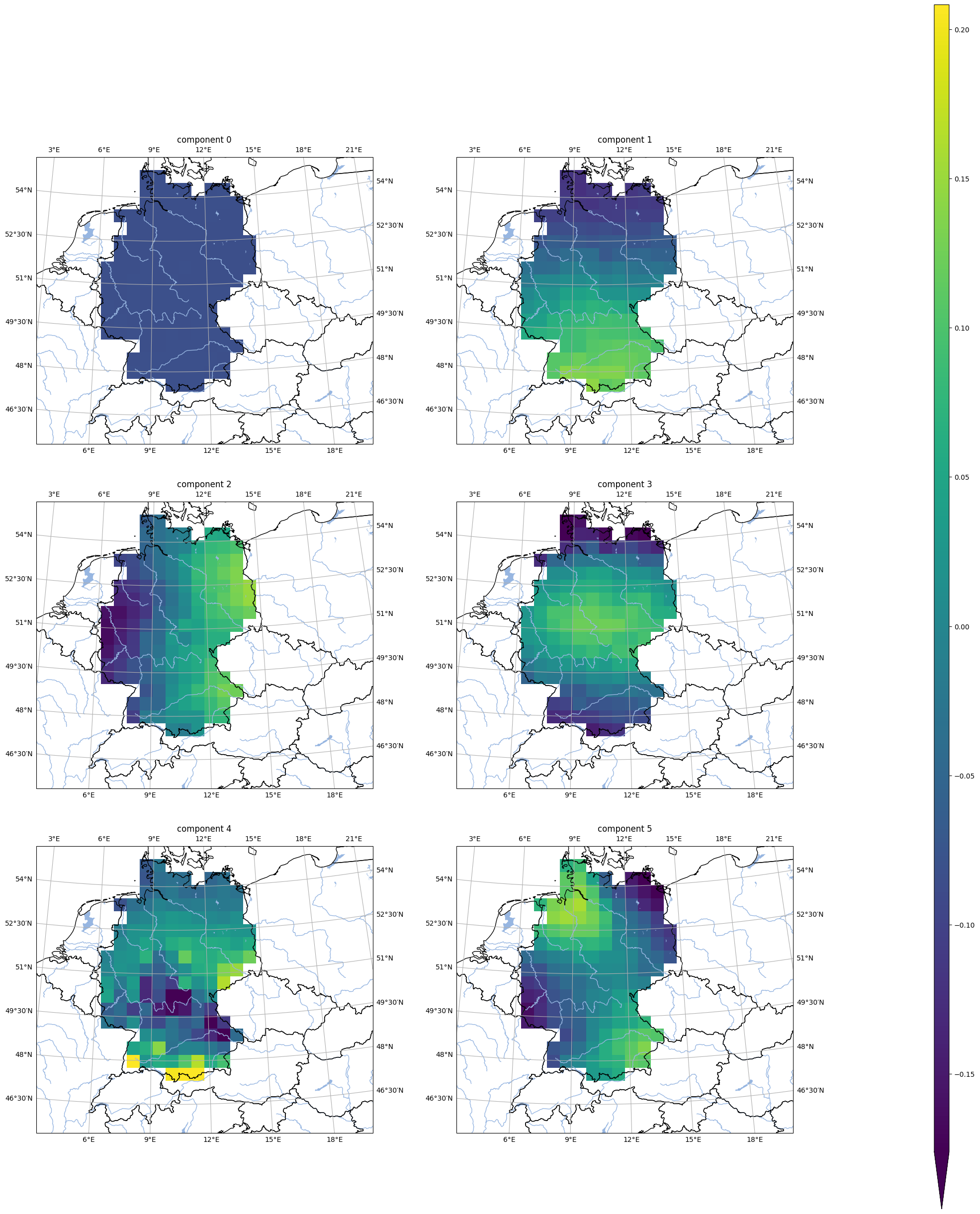
First eigenvectors

analyse.n_maps(
    [
        low_res_training_eigen.isel(nsvs=i).assign_attrs({'label': f'component {i}'})
        for i in np.array(low_res_training_eigen.nsvs[0:6])
    ],
    var='tas',
    crs=area_hr.to_cartopy_crs(),
    ncols=2,
    nrows=3,
    size_inches=(20, 17.*3/2.)
)

<Figure size 640x480 with 0 Axes>

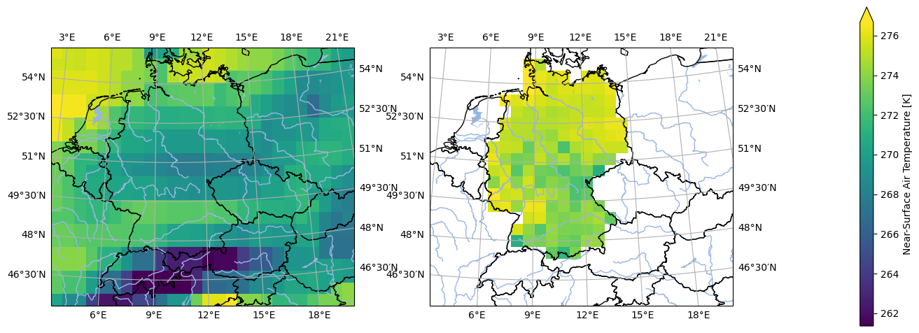
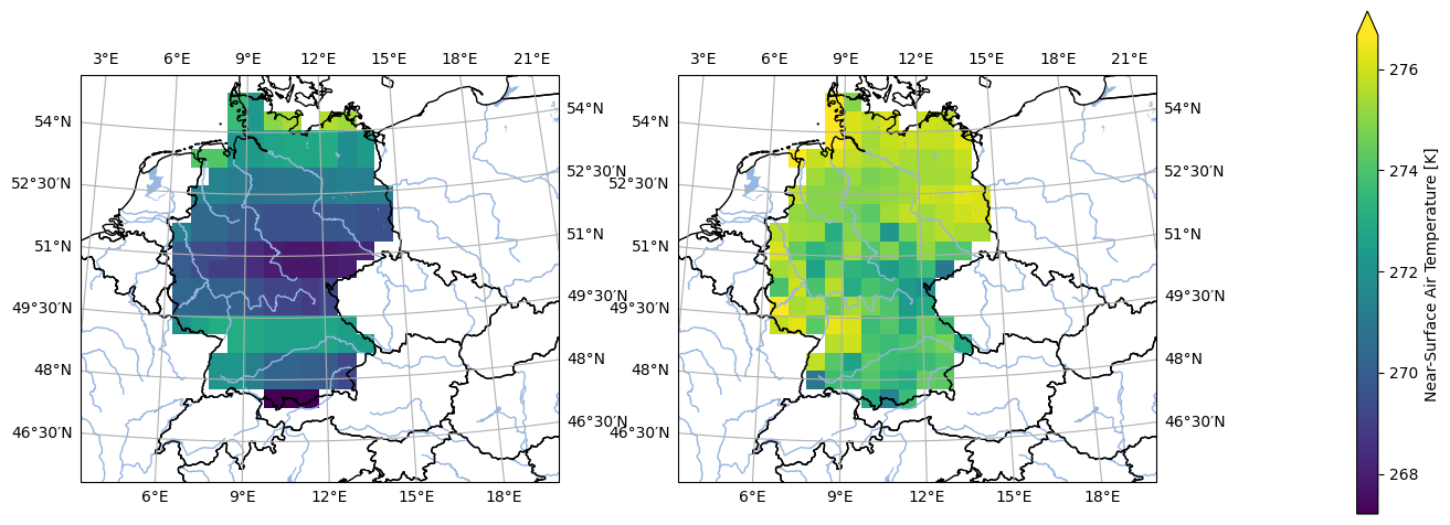
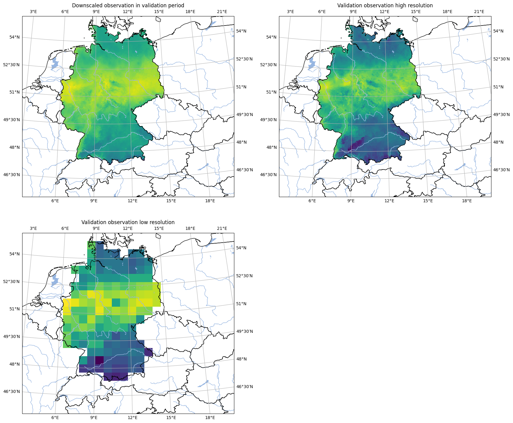
Comparison of downscaling with reference data

analyse.n_maps(
    ds_obs_downscaled.isel(time=300),
    ds_obs_validation_high_res.isel(time=300),
    ds_obs_validation_low_res.isel(time=300),
    var='tas',
    ncols=2,
    nrows=2,
    crs=area_hr.to_cartopy_crs(),
    colorbar=False,
    size_inches=(20, 17)
)

plt.show()

<Figure size 640x480 with 0 Axes>

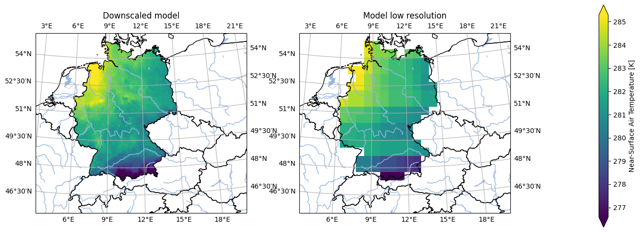
Compare original model and downscaled model

analyse.n_maps(
    ds_mod_downscaled.isel(time=300),
    ds_mod_validation_low_res.isel(time=300),
    var='tas',
    crs='HYR-LAEA-5',
)

plt.show()

<Figure size 640x480 with 0 Axes>