Getting Started#
pyku is an extension built on xarray for handling climate data comprehensively. Its primary aim is to facilitate the reading and manipulation of all climate-related data and metadata. pyku enables tasks such as resampling datetimes, applying masks, polygonizing, reprojection, basic analysis, CMORization, and validation. It is designed to foster collaborative development, emphasizing best practices in code review, style adherence, and deployment.
pyku standardizes our codebase concerning technicalities such as installation and management of dependencies, and resources such as geographic projections, polygons, and color scales.
Collaborative Development#
http://ku.pages.dwd.de/documentation/starter/quality.html
Version Management
Code Review
Code Documentation
Programming style guideline
Unit testing
Integration Testing
CI/CD Pipelines
Core Features#
Handles all tasks associated with geographic projections
Parses and manages all climate-related metadata
Converts polygons and points into raster format
Converts rasters into polygon data
Generates masks from files, creates masks from polygons, and applies them
Visualizes fundamental quantities through plotting
Automatically converts units
Conducts data and metadata integrity checks
Automatically resamples datetime and sets attributes
Dynamically fixes known issues in datasets
Applies CMORization to any dataset
Executes bias correction procedures
Performs downscaling operations
The Mighty Xarray Library#
Xarray makes working with labelled multi-dimensional arrays in Python simple, efficient, and fun!
Ideally, we should avoid writing or re-writing code if it is already available and maintained. For this purpose, pyku is fully integrated with Xarray, extending its datasets with functions focused on handling climate data, particularly the data we use at KU. Since pyku is built within the Xarray framework, it is fully compatible with a large number of high-quality Xarray extensions, allowing us to use them without needing to write and maintain them ourselves. Here are a few examples:
MetPy
MetPy is a collection of tools in Python for reading, visualizing, and performing calculations with weather data.
xclim
xclim is an operational Python library for climate services, providing numerous climate-related indicator tools with an extensible framework for constructing custom climate indicators, statistical downscaling and bias adjustment of climate model simulations, as well as climate model ensemble analysis tools.
xskillscore
Metrics for verifying forecasts
Satpy
Satpy is a python library for reading, manipulating, and writing data from remote-sensing earth-observing satellite instruments.
We load the Xarray and pyku libraries, along with the analyze module from pyku, to perform some plotting during this walk-through.
[1]:
import xarray as xr
import pyku
import pyku.analyse as analyse
Selecting Real-world Data for this Walk-through#
First, we define real-world test data from the pyku.resources module.
[2]:
pyku.list_test_data()
[2]:
['air_temperature',
 'fake_cmip6',
 'cftime_data',
 'hyras',
 'hyras_pr',
 'hyras-tas-monthly',
 'monthly-hyras-files',
 'small_tas_dataset',
 'cosmo-rea6',
 'low-res-hourly-tas-data',
 'hourly-tas',
 'GCM_CanESM5',
 'MPI_ESM1_2_HR_tas',
 'MPI_ESM1_2_HR_pr',
 'tas_hurs',
 'tas_ps_huss',
 'ps_tdew',
 'monthly_eurocordex',
 'global_data',
 'icon_grib_files',
 'icon_grid_file',
 'CCCma_CanESM2_Amon_world']
Checking and Repairing Broken Datasets#
This is generally where we begin our analysis: by going through individual datasets. pyku not only allows us to check datasets for common issues but also tentatively repair on-the-fly any datasets that we use at KU which may be broken.
[3]:
ds = pyku.resources.get_test_data('hyras_pr')
/home/runner/work/pyku/pyku/.venv/lib/python3.12/site-packages/pyku/resources.py:80: UserWarning: Downloading pr_hyras_1_1981_v6-1_de.nc, pr_hyras_1_1982_v6-1_de.nc from https://opendata.dwd.de/climate_environment/CDC/grids_germany/daily/hyras_de/precipitation/to /home/runner/work/pyku/pyku/pyku_cache
  warnings.warn(
Downloading file 'pr_hyras_1_1981_v6-1_de.nc' from 'https://opendata.dwd.de/climate_environment/CDC/grids_germany/daily/hyras_de/precipitation/pr_hyras_1_1981_v6-1_de.nc' to '/home/runner/work/pyku/pyku/pyku_cache'.
Downloading file 'pr_hyras_1_1982_v6-1_de.nc' from 'https://opendata.dwd.de/climate_environment/CDC/grids_germany/daily/hyras_de/precipitation/pr_hyras_1_1982_v6-1_de.nc' to '/home/runner/work/pyku/pyku/pyku_cache'.
As previously mentioned, pyku is built on xarray and leverages its Dataset accessor to seamlessly integrate additional features. These features can be accessed using the pyku accessor, as demonstrated below with the use of the check functions.
[4]:
ds.pyku.check_metadata().query("issue.notna()")
[4]:
| key | value | issue | description | |
|---|---|---|---|---|
| 17 | is_cmor_standard_name | False | pr standard_name is thickness_of_rainfall_amou... | If possible, check if standard name is CMOR co... |
| 18 | is_cmor_long_name | False | pr long_name is Daily Precipitation Sum but th... | Check if long_name is CMOR conform |
| 19 | is_cmor_units | False | pr unit is mm but the expected units is {expec... | Check if units is CMOR conform |
| 33 | time_stamps_are_midnight_or_noon | False | datetimes are ['1981-01-01T06:00:00.000000000'... | Check if all timestamps are midnight or noon |
In the HYRAS data mentioned above, we have identified several issues that can be repaired on-the-fly. Before proceeding, note that you can access the documentation directly in IPython by using the ? command.
[5]:
ds.pyku.check_metadata?
To address the issues identified, you can utilize the pyku standard functions as well as xarray standard functionalities
[6]:
# Convert to cmor units
ds = ds.pyku.to_cmor_units()

# Set the time label at 00:00 every day
ds = ds.assign_coords(time=ds.time.dt.floor('1D'))
[7]:
ds.pyku.check_metadata()
[7]:
| key | value | issue | description | |
|---|---|---|---|---|
| 0 | y_projection_coordinate_exist | True | None | Checking if y projection coordinate available |
| 1 | x_projection_coordinate_exist | True | None | Checking if x projection coordinate available |
| 2 | lat_geographic_coordinate_exist | True | None | Checking if lat geographic coordinate available |
| 3 | lon_geographic_coordinate_exist | True | None | Checking if lon geographic coordinate available |
| 4 | y_projection_coordinate_unit_correct | True | None | Checking if y projection coordinates units |
| 5 | x_projection_coordinate_unit_correct | True | None | Checking if x projection coordinates units |
| 6 | y_projection_coordinate_standard_name_correct | True | None | Checking y projection coordinates standard_name |
| 7 | x_projection_coordinate_standard_name_correct | True | None | Checking x projection coordinates standard_name |
| 8 | lat_geographic_coordinate_unit_correct | True | None | Checking lat geographic coordinate units |
| 9 | lon_geographic_coordinate_unit_correct | True | None | Checking if lat geographic coordinate units |
| 10 | lat_geographic_coordinate_standard_name_correct | True | None | Checking lat geographic coordinate standard_name |
| 11 | lon_geographic_coordinate_standard_name_correct | True | None | Checking lon geographic coordinate standard_name |
| 12 | cf_area_def_readable | True | None | Check if CF projection metadata are readable |
| 13 | area_extent_is_readable | True | None | Check if the area extent can be determined fro... |
| 14 | longitudes_within_180W_and_180E | True | None | Check that the longitudes are within 180 degre... |
| 15 | pr_units_can_be_read | True | None | Check if units can be read automatically |
| 16 | pr | pr | None | NaN |
| 17 | is_cmor_standard_name | True | None | If possible, check if standard name is CMOR co... |
| 18 | is_cmor_long_name | False | pr long_name is Precipitation but the expected... | Check if long_name is CMOR conform |
| 19 | is_cmor_units | True | None | Check if units is CMOR conform |
| 20 | frequency_can_be_inferred_from_data | True | None | Tried to infer frequency from the time labels |
| 21 | frequency_can_be_determined | True | None | Check if frequency can be determined from the ... |
| 22 | geodata_vars | [pr] | None | NaN |
| 23 | geographic_latlon | (lat, lon) | None | NaN |
| 24 | projection_yx | (y, x) | None | NaN |
| 25 | time_dependent_vars | [number_of_stations, pr, time_bnds] | None | NaN |
| 26 | time_bounds_var | time_bnds | None | NaN |
| 27 | spatial_bounds_vars | [y_bnds, x_bnds] | None | NaN |
| 28 | spatial_vertices_vars | [] | None | NaN |
| 29 | crs_var | crs | None | NaN |
| 30 | unidentified_vars | [number_of_stations] | None | NaN |
| 31 | has_time_dimension | True | None | Check if data have a time dimension |
| 32 | time_is_numpy_datetime64_or_cftime | True | None | Check the data type of the time stamps |
| 33 | time_stamps_are_midnight_or_noon | True | None | Check if all timestamps are midnight or noon |
Now we check the data again to make sure that the repair solved the issues.
[8]:
ds.pyku.check_metadata().query("issue.notna()")
[8]:
| key | value | issue | description | |
|---|---|---|---|---|
| 18 | is_cmor_long_name | False | pr long_name is Precipitation but the expected... | Check if long_name is CMOR conform |
Processing Datasets On-the-Fly During Opening#
Xarray allows passing a function to process all files as they are opened, making it an ideal stage for preprocessing! Common tasks include:
Adapting data to your needs
Setting time labels
Standardizing variable names
Standardizing units
To achieve this, we define a function that accepts a dataset, performs operations on it, and returns the modified dataset.
[9]:
def preprocess(ds):

    if 'number_of_stations' in ds.data_vars:
        ds = ds.drop_vars('number_of_stations')

    ds = ds.pyku.to_cmor_units()
    ds = ds.pyku.to_cmor_varnames()
    ds = ds.assign_coords(time=ds.time.dt.floor('1D'))
    ds = ds.pyku.wrap_longitudes()
    ds = ds.sel(time=slice('1981', '1982'))

    return ds
This function can be applied during the file opening process!
Note: pyku offers functions for preprocessing data into a dedicated scratch directory, optionally using parallelism. This functionality is useful for handling large datasets efficiently.
[10]:
# Open the model files
model = pyku.resources.get_test_data('MPI_ESM1_2_HR_pr')

# Open the reference HYRAS files
reference = pyku.resources.get_test_data('hyras_pr')
/home/runner/work/pyku/pyku/.venv/lib/python3.12/site-packages/pyku/resources.py:1717: UserWarning: Downloading NetCDF: s3://esgf-world/CMIP6/CMIP/MPI-M/MPI-ESM1-2-HR/historical/r1i1p1f1/day/pr/gn/v20190710/pr_day_MPI-ESM1-2-HR_historical_r1i1p1f1_gn_19800101-19841231.nc to /home/runner/work/pyku/pyku/pyku_cache
  warnings.warn(f"Downloading NetCDF: {s3_path} to {pyku_data_dir}")
[11]:
model.pyku.check_metadata().query("issue.notna()")
[11]:
| key | value | issue | description | |
|---|---|---|---|---|
| 14 | longitudes_within_180W_and_180E | False | Longitudes not between 180W and 180E | Check that the longitudes are within 180 degre... |
| 18 | is_cmor_long_name | False | pr long_name is Precipitation but the expected... | Check if long_name is CMOR conform |
[12]:
reference.pyku.check_metadata().query("issue.notna()")
[12]:
| key | value | issue | description | |
|---|---|---|---|---|
| 17 | is_cmor_standard_name | False | pr standard_name is thickness_of_rainfall_amou... | If possible, check if standard name is CMOR co... |
| 18 | is_cmor_long_name | False | pr long_name is Daily Precipitation Sum but th... | Check if long_name is CMOR conform |
| 19 | is_cmor_units | False | pr unit is mm but the expected units is {expec... | Check if units is CMOR conform |
| 33 | time_stamps_are_midnight_or_noon | False | datetimes are ['1981-01-01T06:00:00.000000000'... | Check if all timestamps are midnight or noon |
[13]:
model = preprocess(model)
reference = preprocess(reference)
Comparing Datasets#
At this stage, it’s beneficial to compare datasets for fundamental differences. For instance, we may observe that the datasets do not share the same geographic projection.
[14]:
model.pyku.compare_datasets(reference)
[14]:
| key | value | issue | description | |
|---|---|---|---|---|
| 0 | have_same_number_of_pixels_in_y_and_x_directions | False | Datasets do not have the same number of pixels... | Check if number of pixels is the same in the y... |
| 1 | first_dataset_has_time_dimension | True | None | NaN |
| 2 | second_dataset_has_time_dimension | True | None | NaN |
| 3 | first_dataset_datetimes_are_numpy_datetime64 | True | None | NaN |
| 4 | second_dataset_datetimes_are_numpy_datetime64 | True | None | NaN |
| 5 | same_datetimes_in_both_datasets | True | None | NaN |
| 6 | same_rounded_datetimes_in_both_datasets | True | None | NaN |
| 7 | dimensions_names_equal | True | None | NaN |
| 8 | coordinate_names_are_the_same | False | Different keys {'x', 'y'} | NaN |
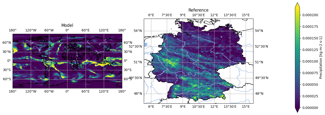
We have a look at the first timestep in the data for a quick sanity check. We spot that the geographic projection used, as well as the masking is not the same.
[15]:
# Set labels
model = model.assign_attrs({'label': 'Model'})
reference = reference.assign_attrs({'label': 'Reference'})

analyse.n_maps(
    model.isel(time=0),
    reference.isel(time=0),
    var='pr'
)
<Figure size 640x480 with 0 Axes>
Managing Geographic Projections#
pyku enables robust handling of geographic projections, which is a core feature of the tool. It supports a wide range of projections, emphasizing standardization across datasets. pyku can manage and write all projection metadata (PROJ string, WKT, CF-conform standard). Refining these standard projection definitions is a continuous and collaborative work.
For a comprehensive list of standardized areas, refer to the documentation or access them directly through pyku.
[16]:
pyku.list_standard_areas()
[16]:
['EUR-44',
 'EUR-11',
 'EUR-6',
 'GER-0275',
 'EPISODES',
 'radolan_wx',
 'DWD_RADOLAN_1100x900',
 'DWD_RADOLAN_900x900',
 'HOSTRADA-1',
 'linet_eqc',
 'euradcom_ps',
 'euradcom_eqc',
 'world_360x180',
 'world_540x270',
 'world_7200x3600',
 'world_3600x1800',
 'world_43200x21600',
 'seamless_europe',
 'seamless_world',
 'seamless_germany',
 'HYR-LCC-1',
 'HYR-LCC-3',
 'HYR-LCC-5',
 'HYR-LCC-125',
 'HYR-LCC-50',
 'HYR-LAEA-1',
 'HYR-LAEA-2',
 'HYR-LAEA-3',
 'HYR-LAEA-5',
 'HYR-LAEA-12.5',
 'HYR-LAEA-50',
 'HYR-LAEA-100',
 'HYR-GER-LAEA-1',
 'HYR-GER-LAEA-2',
 'HYR-GER-LAEA-3',
 'HYR-GER-LAEA-5',
 'HYR-GER-LAEA-12.5',
 'HYR-GER-LAEA-50',
 'HYR-GER-LAEA-100',
 'cerra']
We can project our data onto the HYRAS grid at a 5-kilometer resolution or onto any of the standardized projections listed above.
Note: The HYRAS data are typically already in the projection. Occasionally, the last digits of the georeferencing is not exactly the same depending on what code was used. For simplicity, we reproject the HYRAS data here. The compare functions in pyku will help us determine if the georeferencing alignment is compatible (a check for exact georeferencing alignment will be included in the future).
The code would look like:
projected_model = model.pyku.project('HYR-LAEA-5')
projected_model.pyku.align_georeferencing(reference)
[17]:
# Project to the HYRAS grid
projected_model = model.pyku.project('HYR-LAEA-5')
projected_reference = reference.pyku.project('HYR-LAEA-5')
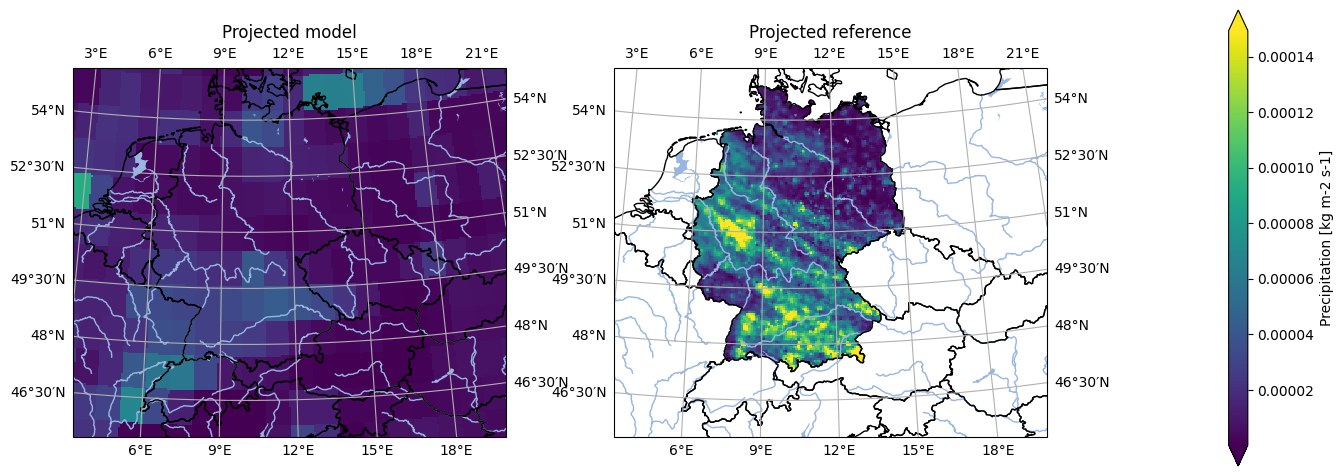
[18]:
# Set labels
projected_model = projected_model.assign_attrs({'label': 'Projected model'})
projected_reference = projected_reference.assign_attrs({'label': 'Projected reference'})

analyse.n_maps(
    projected_model.isel(time=0),
    projected_reference.isel(time=0),
    var='pr',
    crs='HYR-LAEA-5'
)
<Figure size 640x480 with 0 Axes>
Note that during that operation, all geographic projection metadata have been set automatically!
Note the grid mapping attribute, as well as the crs variable
[19]:
projected_model.pr.attrs
[19]:
{'standard_name': 'precipitation_flux',
 'long_name': 'Precipitation',
 'comment': 'includes both liquid and solid phases',
 'units': 'kg m-2 s-1',
 'original_name': 'pr',
 'cell_methods': 'area: time: mean',
 'cell_measures': 'area: areacella',
 'history': '2019-08-25T10:32:27Z altered by CMOR: replaced missing value flag (-9e+33) and corresponding data with standard missing value (1e+20). 2019-08-25T10:32:27Z altered by CMOR: Inverted axis: lat.',
 'grid_mapping': 'crs'}
[20]:
# Note the CRS attributes
projected_model.crs.attrs
[20]:
{'grid_mapping_name': 'lambert_azimuthal_equal_area',
 'longitude_of_projection_origin': 10.0,
 'latitude_of_projection_origin': 52.0,
 'semi_major_axis': 6378137.0,
 'semi_minor_axis': 6356752.31414036,
 'inverse_flattening': 298.257222101,
 'false_easting': 4321000.0,
 'false_northing': 3210000.0,
 'spatial_ref': 'PROJCS["ETRS_1989_LAEA",GEOGCS["GCS_ETRS_1989",DATUM["D_ETRS_1989",SPHEROID["GRS_1980",6378137.0,298.257222101]],PRIMEM["Greenwich",0.0],UNIT["Degree",0.0174532925199433]],PROJECTION["Lambert_Azimuthal_Equal_Area"],PARAMETER["False_Easting",4321000.0],PARAMETER["False_Northing",3210000.0],PARAMETER["Central_Meridian",10.0],PARAMETER["Latitude_Of_Origin",52.0],UNIT["Meter",1.0]]',
 'crs_wkt': 'PROJCS["ETRS_1989_LAEA",GEOGCS["GCS_ETRS_1989",DATUM["D_ETRS_1989",SPHEROID["GRS_1980",6378137.0,298.257222101]],PRIMEM["Greenwich",0.0],UNIT["Degree",0.0174532925199433]],PROJECTION["Lambert_Azimuthal_Equal_Area"],PARAMETER["False_Easting",4321000.0],PARAMETER["False_Northing",3210000.0],PARAMETER["Central_Meridian",10.0],PARAMETER["Latitude_Of_Origin",52.0],UNIT["Meter",1.0]]',
 'proj4': '+proj=laea +lat_0=52 +lon_0=10 +x_0=4321000 +y_0=3210000 +ellps=GRS80 +towgs84=0,0,0,0,0,0,0 +units=m +no_defs +type=crs',
 'proj4_params': '+proj=laea +lat_0=52 +lon_0=10 +x_0=4321000 +y_0=3210000 +ellps=GRS80 +towgs84=0,0,0,0,0,0,0 +units=m +no_defs +type=crs',
 'epsg_code': 'EPSG:3035',
 'long_name': 'DWD HYRAS ETRS89 LAEA grid with 258 columns and 220 rows'}
Masking and Polygon Resources#
A common basic operation involves selecting a region and masking the data. pyku facilitates the standardization and application of polygons for this purpose.
Note: Functions are available to directly obtain mask polygons from a dataset, generate masks in Xarray format, create masks for multiple polygons, or segment datasets into regions. For detailed instructions, please refer to the documentation as this is a brief overview.
First we import the pyku resources module and show the available polygons.
[21]:
import pyku.resources as resources
[22]:
resources.get_polygon_identifiers()
/home/runner/work/pyku/pyku/.venv/lib/python3.12/site-packages/pyku/resources.py:229: FutureWarning: Function 'get_polygon_identifiers' is deprecated. Use 'list_polygon_identifiers'
  warnings.warn(
[22]:
['ne_10m_admin_0_countries',
 'ne_10m_coastline',
 'ne_10m_rivers',
 'ne_10m_lakes',
 'germany',
 'austria',
 'german_states',
 'german_cities',
 'ne_10m_geography_regions_polys',
 'eobs_mask',
 'prudence',
 'natural_areas_of_germany',
 'natural_areas_of_germany_merged4',
 'german_directions',
 'natural_climatic_regions_of_germany']
Here we will select Germany, which is returned as a GeoDataFrame downloaded on-the-fly and on-demand from the original source.
[23]:
germany = resources.get_geodataframe('germany')
germany
[23]:
| featurecla | scalerank | LABELRANK | SOVEREIGNT | SOV_A3 | ADM0_DIF | LEVEL | TYPE | TLC | ADMIN | ... | FCLASS_TR | FCLASS_ID | FCLASS_PL | FCLASS_GR | FCLASS_IT | FCLASS_NL | FCLASS_SE | FCLASS_BD | FCLASS_UA | geometry | |
|---|---|---|---|---|---|---|---|---|---|---|---|---|---|---|---|---|---|---|---|---|---|
| 49 | Admin-0 country | 0 | 2 | Germany | DEU | 0 | 2 | Sovereign country | 1 | Germany | ... | NaN | NaN | NaN | NaN | NaN | NaN | NaN | NaN | NaN | MULTIPOLYGON (((13.81572 48.76643, 13.78586 48... |
1 rows × 169 columns
And now we can apply the mask directly to our datasets.
[24]:
masked_model = projected_model.pyku.apply_mask(germany)
masked_reference = projected_reference.pyku.apply_mask(germany)
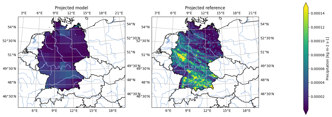
A quick sanity check now shows us the projected and masked datasets
[25]:
# Set labels
masked_model = masked_model.assign_attrs({'label': 'Projected model'})
masked_reference = masked_reference.assign_attrs({'label': 'Projected reference'})

analyse.n_maps(
    masked_model.isel(time=0),
    masked_reference.isel(time=0),
    var='pr',
    crs='HYR-LAEA-5'
)
<Figure size 640x480 with 0 Axes>
Basic Plotting#
pyku features an analyse module designed for simple plotting and dataset exploration. While currently intended for basic visualization rather than comprehensive analysis, future developments may expand its capabilities in that direction. Given the small size of the dataset used here, it can be fully loaded into memory for optimal performance in this notebook. However, pyku can handle datasets of any size without limitations.
[26]:
masked_model = masked_model.compute()
masked_reference = masked_reference.compute()
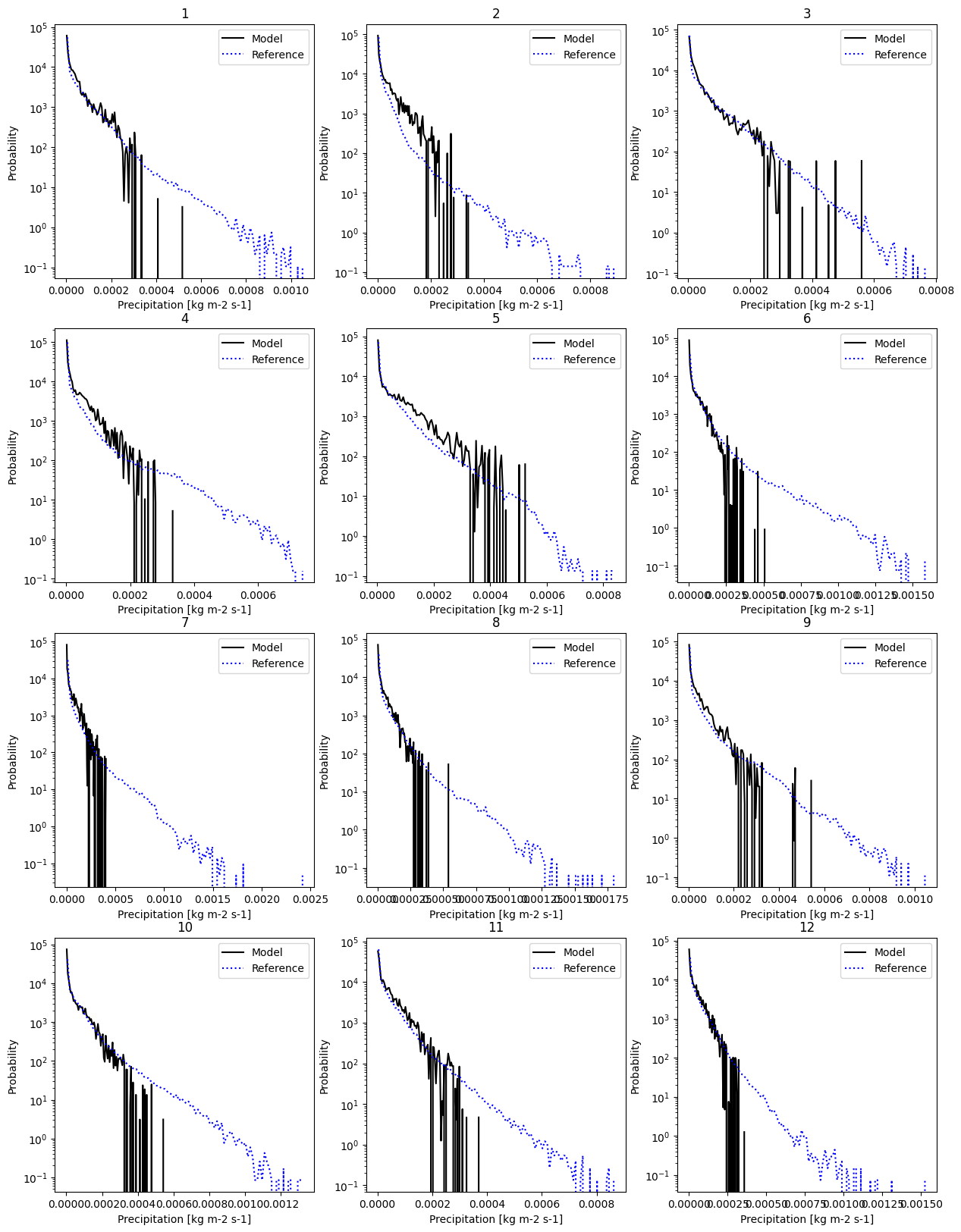
And here we can have a look for example at the monthly probability distribution function. We set the label of the data and plot.
[27]:
# Set labels
masked_model = masked_model.assign_attrs({'label': 'Model'})
masked_reference = masked_reference.assign_attrs({'label': 'Reference'})

analyse.monthly_pdf(
    masked_model,
    masked_reference,
    var='pr',
    nbins=100,
    yscale='log'
)
<Figure size 640x480 with 0 Axes>
Resampling Datetimes#
The functionnality for resampling datetimes is certainly of generic interest. First, let’s examine the dataset and isolate the temperature data. Note that the dataset includes time_bounds and crs as data variables.
[28]:
masked_model.data_vars
[28]:
Data variables:
    pr         (time, y, x) float32 166MB nan nan nan nan ... nan nan nan nan
    time_bnds  (time, bnds) datetime64[ns] 12kB 1981-01-01 ... 1983-01-01
    crs        int32 4B 1
If we were to select the temperature using the standard Xarray functions, we would lose that information.
[29]:
masked_model[['pr']].data_vars
[29]:
Data variables:
    pr       (time, y, x) float32 166MB nan nan nan nan nan ... nan nan nan nan
pyku offers an alternative selection method to obtain a dataset with all the relevant climate data information.
[30]:
pr_data = masked_model.pyku.get_geodataset('pr')
pr_data.data_vars
[30]:
Data variables:
    pr         (time, y, x) float32 166MB nan nan nan nan ... nan nan nan nan
    crs        int32 4B 1
    time_bnds  (time, bnds) datetime64[ns] 12kB 1981-01-01 ... 1983-01-01
We can now resample the data to a monthly frequency, specifying the resampling method (here, using the sum). The time bounds have been automatically adjusted during resampling.
[31]:
pr_data.pyku.resample_datetimes(how='sum', frequency='1MS')
[31]:
<xarray.Dataset> Size: 12MB
Dimensions:    (time: 24, bnds: 2, y: 220, x: 258)
Coordinates:
  * time       (time) datetime64[ns] 192B 1981-01-01 1981-02-01 ... 1982-12-01
  * y          (y) float64 2kB 3.586e+06 3.582e+06 ... 2.496e+06 2.492e+06
  * x          (x) float64 2kB 3.808e+06 3.814e+06 ... 5.088e+06 5.094e+06
    lat        (y, x) float64 454kB 55.13 55.13 55.14 ... 45.09 45.08 45.08
    lon        (y, x) float64 454kB 1.95 2.028 2.106 2.184 ... 19.7 19.76 19.83
Dimensions without coordinates: bnds
Data variables:
    time_bnds  (time, bnds) datetime64[ns] 384B 1981-01-01 ... 1983-01-01
    pr         (time, y, x) float64 11MB 0.0 0.0 0.0 0.0 0.0 ... 0.0 0.0 0.0 0.0
    crs        int32 4B 1
Attributes: (12/49)
    Conventions:            CF-1.7 CMIP-6.2
    activity_id:            CMIP
    branch_method:          standard
    branch_time_in_child:   0.0
    branch_time_in_parent:  0.0
    contact:                cmip6-mpi-esm@dkrz.de
    ...                     ...
    variant_label:          r1i1p1f1
    license:                CMIP6 model data produced by MPI-M is licensed un...
    cmor_version:           3.5.0
    tracking_id:            hdl:21.14100/de725be4-bcb0-41fb-96e9-0e61de57daaf
    label:                  Model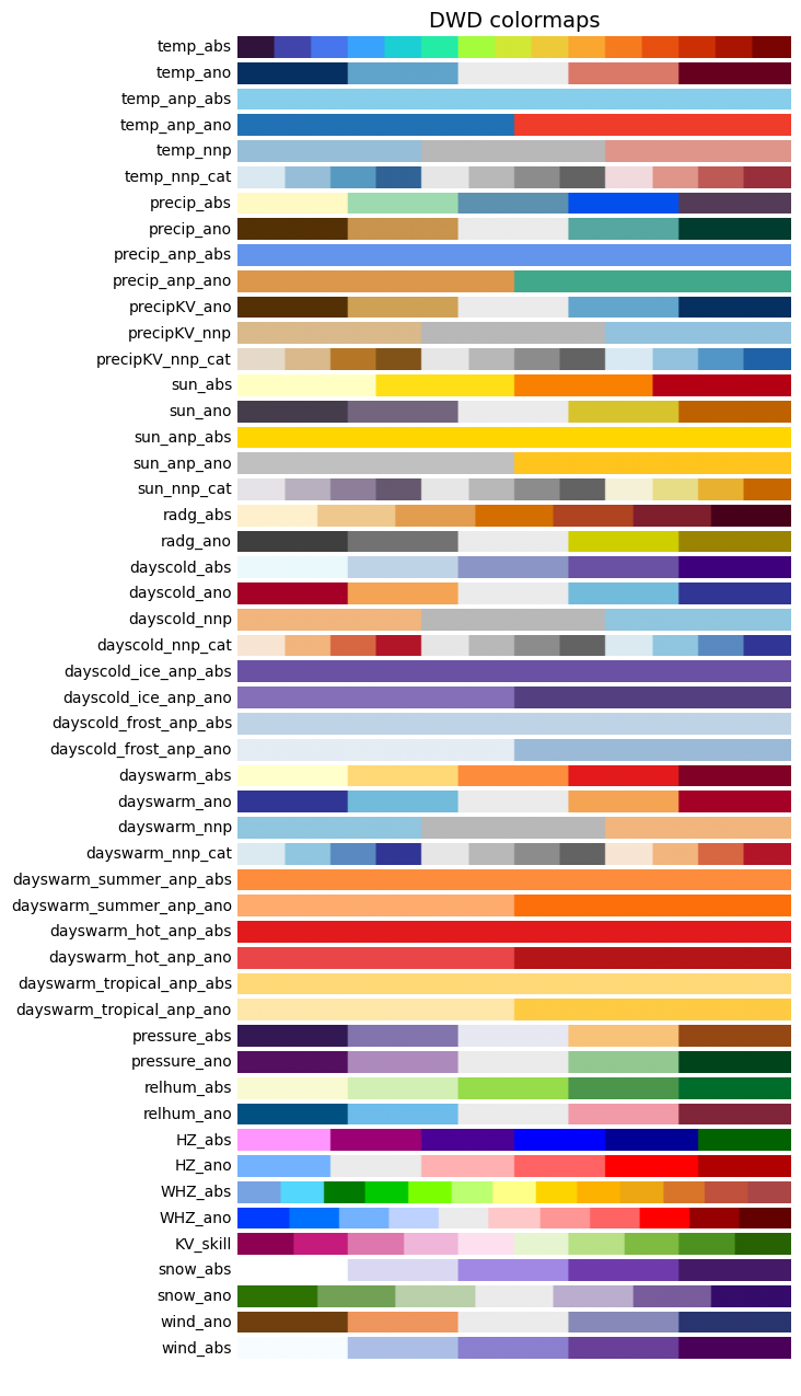
CORDEX_domain: undefinedThe KU Colormap#
pyku includes the KU standard colormap for consistent use across our projects. Implementing this colormap aims to streamline our workflow by eliminating the need to define the colormap in each code individually. By importing the colormap module, updating to the latest version via pip install --upgrade ensures all codes are synchronized.
Let’s begin by importing the module and visualizing all available colormaps.
[32]:
import pyku.colormaps as colormaps
[33]:
colormaps.plot_colormaps(kind='original')
Once we’ve selected a colormap of interest, we can apply it using the cmap keyword. In Python, cmap from Matplotlib serves as the de facto standard for colormaps, compatible with virtually any plotting library.
[34]:
mycolormap = colormaps.get_cmap('temp_ano', kind='original')
For example, the plotting routines in the analyse module can take any relevant matplotlib keywords, and in particular the cmap keyword.
[35]:
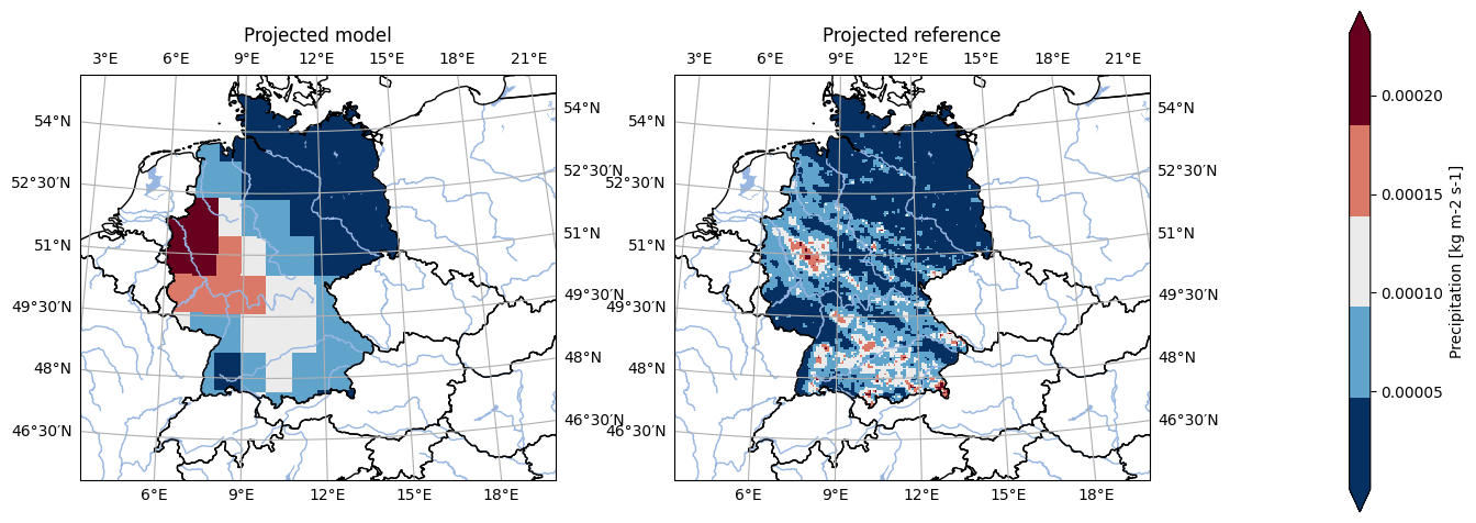
# Set labels
masked_model = masked_model.assign_attrs({'label': 'Projected model'})
masked_reference = masked_reference.assign_attrs({'label': 'Projected reference'})

analyse.n_maps(
    masked_model.isel(time=10),
    masked_reference.isel(time=0),
    cmap=mycolormap,
    var='pr',
    crs='HYR-LAEA-5'
)
<Figure size 640x480 with 0 Axes>