LOESS filter

The Loess filter function pyku.loess.loess can be used for standalone time-series and values arrays and pyku.compute.calc_loess is designed to take a xr.Dataset as input (while under the hood making use of the first)

Standalone example

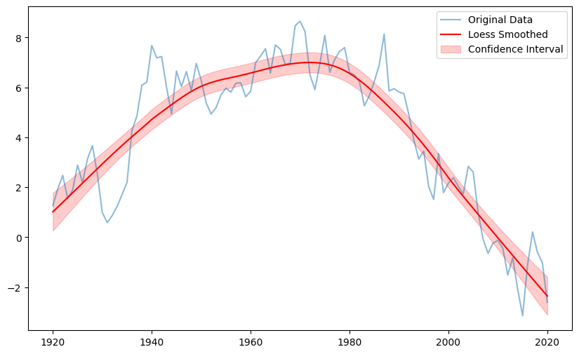
You can pass two arrays to the pyku.loess.loess function and directly estimate the filtered data with DWD-configuration standards of the loess filter. The first array can be for example a numpy array (of time steps) or a pandas date_range array. The second array is your values. The need to be of the same lenght and for the default configuration of length > than 42 (since otherwise the span of size 42 wouldnt make sense.)

import pandas as pd
import numpy as np
import matplotlib.pyplot as plt

from pyku.loess import loess

x = pd.date_range(start='1920-01-01', periods=101, freq='YS')
y = np.random.randn(101).cumsum()

result = loess(x, y)
print("Smoothed values:", result.df)


plt.figure(figsize=(10, 6))
plt.plot(x, y, label='Original Data', alpha=0.5)
plt.plot(x, result.values, label='Loess Smoothed', color='red')
plt.fill_between(x, result.lower, result.upper, color='red', alpha=0.2, label='Confidence Interval')
plt.legend()
plt.show()

Smoothed values:           time    values     upper     lower
0   1920-01-01  1.018023  1.776545  0.259501
1   1921-01-01  1.207414  1.928551  0.486276
2   1922-01-01  1.397363  2.082425  0.712300
3   1923-01-01  1.588307  2.238584  0.938030
4   1924-01-01  1.780092  2.396968  1.163215
..         ...       ...       ...       ...
96  2016-01-01 -1.430797 -0.813982 -2.047612
97  2017-01-01 -1.663775 -1.013467 -2.314082
98  2018-01-01 -1.895108 -1.210013 -2.580203
99  2019-01-01 -2.125353 -1.404182 -2.846525
100 2020-01-01 -2.354518 -1.596064 -3.112972

[101 rows x 4 columns]

A trend can be estimated by passing a target and a reference to the objects trend function. Those can be either given as indices (with index=True (default)) or as time steps, where the type of the time steps need to have the same type as the original used time series for the estimation of the loess curve. Note, that the right border is inclusive for the time-based slicing, but not for the index based.

Mixing indexed and time-based indexing is not possible.

Lets have a look into that with examples:

x = pd.date_range(start='1881-01-01', periods=144, freq='YS')
y = np.random.randn(144).cumsum()

result = loess(x, y)

# Using time-based target and reference periods
loess_trend = result.trend(target=pd.Timestamp('2024-01-01'),
                           ref=(pd.Timestamp('1881-01-01'), pd.Timestamp('1910-01-01')),
                           index=False)
print("Trend result:", loess_trend)
# Expected output: (Timestamp('1950-01-01 00:00:00'), trend_value)

# Using index-based target and reference periods
loess_trend_index = result.trend(target=143, ref=(0,30), index=True)
print("Trend result (index):", loess_trend_index)
# Expected output: (Timestamp('1950-01-01 00:00:00'), trend_value)


# If using pandas.DatetimeIndex, you can also use datetime objects to indicate target and reference periods
import datetime

result = loess(x, y)

loess_trend = result.trend(target=datetime.datetime(2024, 1, 1),
                           ref=(datetime.datetime(1881, 1, 1), datetime.datetime(1910, 1, 1)),
                           index=False)
print("Trend result (datetime):", loess_trend)

Trend result: (Timestamp('2024-01-01 00:00:00'), -5.591632896550365)
Trend result (index): (Timestamp('2024-01-01 00:00:00'), -5.591632896550365)
Trend result (datetime): (Timestamp('2024-01-01 00:00:00'), -5.591632896550365)

From a xr.Dataset

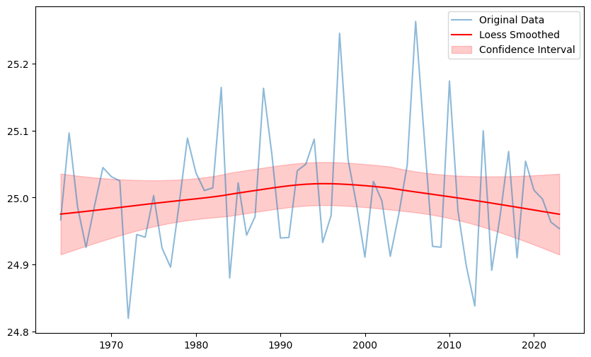
there is also a calc_loess function that allows to calculate the loess-filter along each grid point of lat-lon (or any other identifieable geographics). If you xr.Dataset has more than one variable you will need to pass the variable name to the calc_loess function. Loess gets now calculated for each grid point separately and a new dataset with variables {var}_loess, {var}_loess_lower and {var}_loess_upper gets returned.

import matplotlib.pyplot as plt

import pyku.resources
from pyku.loess import calc_loess

# Generate some example data. 60 years of daily data on a 5x5 regular grid
ds = pyku.resources.generate_fake_cmip6_data(ntime=60, nlat=36, nlon=72, freq='D')

result = calc_loess(ds, var='tas')

ts = (
        ds['tas'].resample(time='1YS')
        .mean(dim='time', keep_attrs=True)
    )

plt.figure(figsize=(10, 6))
plt.plot(ts.time, ts.isel(lon=0,lat=0), label='Original Data', alpha=0.5)
plt.plot(result.time, result['tas_loess'].isel(lon=0,lat=0), label='Loess Smoothed', color='red')
plt.fill_between(result.time,
                 result['tas_loess_lower'].isel(lon=0,lat=0),
                 result['tas_loess_upper'].isel(lon=0,lat=0),
                 color='red', alpha=0.2, label='Confidence Interval')
plt.legend()
plt.show()